简介

注释：

单行注释：– 或 #

多行注释：/**/

SQL分类：

DDL：数据定义语言，定义数据库对象（数据库，表，字段）。

DML：数据操作语言，对数据进行增删改。

DQL：数据查询语言，查询数据表的记录。

DCL：数据控制语言，创建数据库用户，控制数据库访问权限。

DDL

查询所有数据库：SHOW DATABASES;

查询当前数据库：SELECT DATABASE();

创建数据库：CREATE DATABASE [IF NOT EXISTS] 数据库名 [DEFAULT CHARSET 字符集] [COLLATE 排序规则];

删除数据库：DROP DATABASE [IF EXISTS] 数据库名;

切换数据库：USE 数据库名;

查询当前数据库中的所有表：SHOW TABLES;

查询表结构：DESC 表名;

查询指定表的建表语句：SHOW CREATE TABLE 表名;

创建表：

1
2
3
4
5
6

CREATE TABLE 表名(
  字段1 字段1类型 [COMMENT 字段注释],
  字段2 字段2类型 [COMMENT 字段注释],
  ...
  字段n 字段n类型 [COMMENT 字段注释]
) [表注释];

修改表：

• 添加字段：ALTER TABLE 表名 ADD 字段名 类型（长度）[COMMENT 注释] [约束];
• 修改数据类型： ALTER TABLE 表名 MODIFY 字段名 新数据类型（长度）;
• 修改字段名和字段类型：ALTER TABLE 表名 CHANGE 旧字段名 新字段名 类型（长度） [COMMENT 注释] [约束];
• 删除字段：ALTER TABLE 表名 DROP 字段名;
• 修改表名：ALTER TABLE 表名 RENAME TO 新表名;
• 删除表：DROP TABLE [IF EXISTS] 表名;
• 删除指定表，并重新创建该表：TRUNCATE TABLE;

示例：

现有一张用户信息表 user_info，其中包含多年来在平台注册过的用户信息。

请在用户信息表，字段 level 的后面增加一列最多可保存 15 个汉字的字段 school；并将表中 job 列名改为 profession，同时 varchar 字段长度变为 10；achievement 的默认值设置为 0。

1
2
3

ALTER TABLE user_info ADD school varchar(15) AFTER `level`;
ALTER TABLE user_info CHANGE job profession varchar(10);
ALTER TABLE user_info CHANGE COLUMN achievement achievement int DEFAULT 0;

DML

给指定字段添加数据：INSERT INTO 表名 (字段1，字段2，...) VALUES (值1，值2);

给全部字段添加数据：INSERT INTO 表名 VALUES (值1，值2);

批量添加数据：

1
2

INSERT INTO 表名 (字段1，字段2，...) VALUES (值1，值2, ...), (值1，值2, ...), (值1，值2, ...);
INSERT INTO 表名 VALUES (值1，值2，...), (值1，值2，...), (值1，值2，...);

[!NOTE]

将多次单行插入合并为一次批量插入（multi-row INSERT）能够显著提升性能，主要原因包括：

• 减少网络往返次数，降低客户端与服务器的通信开销；
• 减少 SQL 解析与执行计划的开销，只需对一条语句进行解析与优化；
• 减少事务与日志写入开销，合并写入二进制日志（binlog）和 InnoDB 重做日志；
• 优化索引更新，批量更新索引比单次多次更新更高效；
• 降低锁竞争与事务开销，减少锁的申请与释放次数；
• 充分利用 InnoDB 的 Group Commit 机制，进一步减少磁盘刷新次数。

示例：

现有一张试卷作答记录表exam_record，结构如下表，其中包含多年来的用户作答试卷记录，由于数据越来越多，维护难度越来越大，需要对数据表内容做精简，历史数据做备份。

1
2
3
4

INSERT INTO exam_record_before_2021(uid, exam_id, start_time, submit_time, score)
SELECT uid, exam_id, start_time, submit_time, score
FROM exam_record
WHERE YEAR(submit_time) < '2021';

现在有一套ID为9003的高难度SQL试卷，时长为一个半小时，请你将 2021-01-01 00:00:00 作为发布时间插入到试题信息表examination_info（其表结构如下图），不管该ID试卷是否存在，都要插入成功，请尝试插入它。

1
2
3
4
5
6
7

REPLACE INTO examination_info
VALUES(NULL,9003,'SQL','hard',90,'2021-01-01 00:00:00');

DELETE FROM examination_info
WHERE exam_id=9003;
INSERT INTO examination_info
VALUES(NULL,9003, 'SQL','hard', 90, '2021-01-01 00:00:00');

修改数据：UPDATE 表名 SET 字段1=值1， 字段2=值2，... [WHERE 条件];

删除数据：DELETE FROM 表名 [WHERE 条件];

[!NOTE]

DELETE 与 TRUNCATE 的区别

操作类型

• DELETE：属于 DML（数据操作语言），需要逐行删除数据，并记录每一行的删除操作。删除后需要手动提交事务。
• TRUNCATE：属于 DDL（数据定义语言），直接释放表的所有数据页，然后重新初始化表，速度更快。

日志记录

• DELETE：会记录每一行的删除操作到 binlog，用于事务回滚和主从同步。
• TRUNCATE：只记录表的重建操作，不记录逐行删除，日志量较小。

重置 AUTO_INCREMENT

• DELETE：不会重置自增值，下一次插入时继续从当前最大值递增。
• TRUNCATE：会重置自增值为初始值。

外键约束

• DELETE：可以针对有外键约束的表逐行删除，受外键规则影响。
• TRUNCATE：不能直接操作有外键约束的表，否则会报错。

当一个表中有大量的 DELETE 操作时，你会采取哪些措施来优化性能或管理存储空间？

1. 如果需要清空整张表，用 TRUNCATE 或 DROP。
2. 如果 DELETE 操作是高频行为，考虑使用 分区表 或 分表。
3. 如果需要保留数据历史，使用 软删除。
4. 定期使用 OPTIMIZE TABLE 或分批 DELETE 来回收空间。

示例：

请删除exam_record表中未完成作答或作答时间小于5分钟整的记录中，开始作答时间最早的3条记录。

1

delete from exam_record where date_add(start_time, interval 5 minute) > submit_time or submit_time is null limit 3;

请删除exam_record表中所有记录，并重置自增主键。

1

truncate table exam_record;

更新语句的执行过程

在执行 UPDATE 时，InnoDB 会先按照 WHERE 条件对匹配的记录及其前后间隙加上 next-key 锁，以防幻读；然后从缓冲池中将数据页加载到内存，先在 Undo 日志中记录修改前的值（用于回滚和 MVCC），再将更新操作以物理日志的形式写入 Redo 日志并将数据页标记为“脏页”。之后 MySQL 采用两阶段提交：第一阶段将 Redo 日志持久化并标记为 prepare 状态，第二阶段将事务的所有变更以逻辑或行事件写入 Binlog 并执行 fsync，最后将 Redo 日志标记为已提交并释放锁，从而保证 Redo 与 Binlog 的原子一致性。

MySQL 在执行更新语句时，在服务层执行语句的解析和执行，在引擎层执行数据的提取和存储；在服务层对 binlog 进行写入，在引擎层对 redo log 进行写入。

事务的两阶段提交

这是 MySQL 中保证数据一致性和持久性的关键机制。

1. prepare 阶段：记录事务的变更到 redo log，并标记为 prepare 状态。
2. binlog 写入：将对应的 SQL 语句写入 binlog。
3. commit 阶段：将 redo log 中对应的日志条目标记为 commit 状态，并完成整个提交过程。

事务不一致的处理

**情况一：**系统在 redo log 标记为 prepare 之后崩溃。这种情况下，事务已经记录到 redo log 中，但可能还未写入 binlog。恢复时，InnoDB 会检查 redo log 中的 prepare 状态。如果找到这样的记录，会继续检查 binlog。

1. 如果 binlog 中没有找到对应的记录，说明事务未提交，InnoDB 会回滚事务，确保数据一致性。
2. 如果 binlog 中找到了对应的记录，说明事务已提交，InnoDB 会完成提交过程，确保数据一致性。

**情况二：**系统在 binlog 写入后但在 redo log commit 前崩溃。在这种情况下，事务已经写入了 binlog，但未完成在 redo log 中的 commit 标记。恢复时，InnoDB 会首先检查 redo log，如果发现 prepare 状态的记录且 binlog 中有对应的记录，InnoDB 会将事务标记为 commit 状态并完成提交，这确保了事务的一致性和持久性。

DQL

查询多个字段：

1
2

SELECT 字段1，字段2，字段3... FROM 表名;
SELECT * FROM 表名;

设置别名：SELECT 字段1 [AS 别名1]，字段2[AS 别名2] ... FROM 表名;

去除重复记录：SELECT DISTINCT 字段列表 FROM 表名;

聚合函数：SELECT 聚合函数(字段) FROM 表名;

以上 SQL 语句将一列数据作为一个整体，进行纵向计算。NULL 不参与所有聚合函数运算。

分组查询：SELECT 字段列表 FROM 表名 [WHERE 条件] GROUP BY 分组字段名 [HAVING 分组后过滤条件];

[!NOTE]

WHERE 和 HAVING 区别

• 执行时机不同：WHERE 是分组之前进行过滤；HAVING 是分组之后进行过滤。
• 判断条件不同：WHERE 不能对聚合函数进行判断，HAVING 可以。
• 执行顺序：WHERE > 聚合函数 > HAVING

排序查询：SELECT 字段列表 FROM 表名 ORDER BY 字段1 排序方式1, 字段2 排序方式2;

排序方式：ASC 升序（默认），DESC 降序。

如果是多字段排序，当第一个字段值相同时，才会根据第二个字段进行排序。

分页查询：SELECT 字段列表 FROM 表名 LIMIT 起始索引，查询记录数;

起始索引从0开始，起始索引 =（查询页码 - 1）* 每页显示记录数;

SELECT 查询执行顺序

1. FROM：对 FROM 子句中的左表和右表执行笛卡儿积（Cartesianproduct），产生虚拟表 VT1。
2. ON：对虚拟表 VT1 应用 ON 筛选，只有那些符合的行才被插入虚拟表 VT2 中。
3. JOIN：如果指定了 OUTER JOIN（如 LEFT OUTER JOIN、RIGHT OUTER JOIN），那么保留表中未匹配的行作为外部行添加到虚拟表 VT2 中，产生虚拟表 VT3。如果 FROM 子句包含两个以上表，则对上一个连接生成的结果表 VT3 和下一个表重复执行步骤 1）～步骤 3），直到处理完所有的表为止。
4. WHERE：对虚拟表 VT3 应用 WHERE 过滤条件，只有符合的记录才被插入虚拟表 VT4 中。
5. GROUP BY：根据 GROUP BY 子句中的列，对 VT4 中的记录进行分组操作，产生 VT5
6. CUBE | ROLLUP：对表 VT5 进行 CUBE 或 ROLLUP 操作，产生表 VT6。
   1. CUBE：生成所有可能组合的汇总，包括每个维度的组合。适用于多维数据分析。
   2. ROLLUP：生成层级汇总，从详细级别到总体总和。适用于生成部分汇总数据。
7. HAVING：对虚拟表 VT6 应用 HAVING 过滤器，只有符合的记录才被插入虚拟表 VT7 中。
8. SELECT：第二次执行 SELECT 操作，选择指定的列，插入到虚拟表 VT8 中。
9. DISTINCT：去除重复数据，产生虚拟表 VT9。
10. ORDER BY：将虚拟表 VT9 中的记录按照进行排序操作，产生虚拟表 VT10。
11. LIMIT：取出指定行的记录，产生虚拟表 VT11，并返回给查询用户。

DQL 语句的执行过程

1. 客户端通过 TCP 连接发送 DQL 到 MySQL 服务器。
2. 连接器开始处理该请求，包括建立连接、权限验证等。
3. 解析器进行词法分词和语法分析，生成抽象语法树 AST 或解析树，同时检查 SQL 语法合法性和基本语法错误。在生成 AST 后，解析器将数据库名、表名和列名等标识符与内部数据字典中的对象进行映射，并对引用的对象执行权限检查，只有在用户拥有相应权限时，才允许继续执行。
4. 优化器基于成本模型，对解析树进行查询重写（如谓词下推、视图展开）和逻辑优化，然后评估多种访问路径：全表扫描 vs 索引扫描、Nested Loop Join vs Hash Join 等，计算各方案的成本并选择最优执行计划，该计划以具体的物理操作算子（索引扫描、排序、聚合）为粒度进行组合。
5. 执行器根据优化器生成的执行计划，调用相应的存储引擎接口，逐步执行算子操作（TableScan、IndexScan、Join、Sort），并在内存中构建最终的结果集。
6. 对于 InnoDB 引擎，普通 SELECT 语句采用多版本并发控制（MVCC），从缓冲池内查找 Undo 日志中保存的历史版本来重建查询时刻的数据快照，若未命中则从磁盘读取并加载到缓冲池，同时维护 LRU 链表。
7. 执行器完成结果集的生成后，通过 Protocol 层将数据逐行或一次性打包返回给客户端。

DCL

查询用户：

1
2

USE mysql;
SELECT * FROM user;

创建用户：CREATE USER '用户名'@'主机名' IDENTIFIED BY '密码';

修改用户密码：ALTER USER '用户名'@'主机名' IDENTIFIED WITH mysql_native_password BY '新密码';

删除用户：DROP USER '用户名'@'主机名';

查询权限：SHOW GRANTS FOR '用户名'@'主机名';

授予权限：GRANT 授权列表 ON 数据库名.表名 TO '用户名'@'主机名';

撤销权限：REVOKE 权限列表 ON 数据库名.表名 FROM '用户名'@'主机名';

[!NOTE]

主机名可使用 % 通配。

多个权限之间使用逗号分隔。

数据库名和表名可使用 * 进行通配，代表所有。

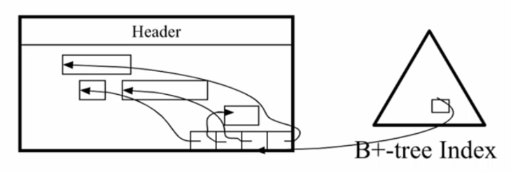
Each page consits of the header, the record space and a pointer array. Each slot in this array points to a record within the page.

A record is located by providing its page address and the slot number. The combination is called RID.

Life Cycle of a record:

Insert: Find an empty space to put it and set a slot at the very end of the page to point to it.

Delete: Remove the record and reclaim this space, set its slot number to null. When there are too many garbage slots, the system will drop the index structure, do reorganization on this disk page by removing all null slots, and reconstruct the index structure from scratch.

Non-clustered Index: the data of the disk page is independent of the bucket or leaf node of index.

Clustered Index: the data of the disk page resides within the bucket or leaf node of index.

Hash Index: the item in buckets is not ordered by the attribute value of index.

B+Tree Index: the item in leaf nodes is ordered by the attribute value of index.

• Primary Index: the data in the disk page is ordered.
• Secondary Index: the data in the disk page is not ordered.

Reference: https://www.vldb.org/conf/1990/P481.PDF

Overview

The HRPS declusters a relation into fragment based on the following criteria:

• Each fragment contains approximately FC tuples.
• Each fragment contains a unique range of values of the partitioning attribute.

The variable FC is determined based on the processing capability of the system and the resource requirements of the queries that access the relation (rather than the number of processors in the configuration).

A major underlying assumption of this partitioning strategy is that the selection operators which access the database retrieve and process the selected tuples using either a range predicate or an equality predicate.

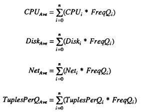
For each query Qi, the workload defines the CPU processing time (CPUi), the Disk Processing Time (Diski), and the Network Processing time (Neti) of that query. Observe that these times are determined based on the resource requirements of each individual query and the processing capability of the system. Each query retrieves and processes (TuplesPerQi) tuples from the database. Furthermore, we assume that the workload defines the frequency of occurrence of each query (FreqQi).

Rather than describing the HRPS with respect to each query in the workload, we deline an average query (Qavg) that is representative of all the queries in the workload. The CPU, disk and network processing quanta for this query are:

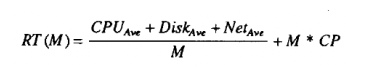
Assume that a single processor cannot overlap the use of two resources for an individual query. Thus, the execution time of Qavg on a single processor in a single user environment is:

As more processors are used for query execution, the response time decreases. However, this also incurs additional overhead, represented by the variable CP, which refers to the cost of coordinating the query execution across multiple processors (e.g., messaging overhead). The response time of the query on M processors can be described by the following formula:

In a single-user environment, both HRPS and range partitioning perform similarly because they both efficiently execute the query on the required processor. However, in a multi-user environment, the range partitioning strategy is likely to perform better because it can distribute the workload across multiple processors, improving system throughput. In contrast, HRPS might not utilize all available processors as effectively, potentially leading to lower throughput.

Instead of M representing the number of processors over which a relation should be declustered, M is used instead to represent the number of processors that should participate in the execution of Qavg. Since Qavg processes TuplesPerQavg tuples, each fragment of the relation should contain FC = TuplesPerQavg / M tuples.

The process of fragmenting and distributing data in HRPS:

1. Sorting the relation: The relation is first sorted based on the partitioning attribute to ensure each fragment contains a distinct range of values.
2. Fragmentation: The relation is then split into fragments, each containing approximately FC tuples.
3. Round-robin distribution: These fragments are distributed to processors in a round-robin fashion, ensuring that adjacent fragments are assigned to different processors (unless the number of processors N is less than the required processors M).
4. Storing fragments: All the fragments for a relation on a given processor are stored in the same physical file.
5. Range table: The mapping of fragments to processors is maintained in a one-dimensional directory called the range table.

This method ensures that at least M processors and at most M + 1 processors participate in the execution of a query.

M = N：系统和查询需求匹配，HRPS 调度所有处理器，达到最大并行度和最优性能。

M < N：HRPS 只调度一部分处理器执行查询，减少通信开销，但部分处理器资源可能闲置。

M > N：HRPS 将多个片段分配给处理器，尽量利用所有处理器，但每个处理器负担加重，查询执行速度可能受到影响。

HRPS in this paper supports only homogeneous nodes.

Questions

How does HRPS decide the ideal degree of parallelism for a query?

HRPS (Hybrid-Range Partitioning Strategy) decides the ideal degree of parallelism by analyzing the resource requirements of the query, such as CPU, disk I/O, and communication costs. It calculates the optimal number of processors (denoted as M) based on these factors. The strategy strikes a balance between minimizing query response time and avoiding excessive overhead from using too many processors.

Why is it not appropriate to direct a query that fetches one record using an index structure to all the nodes of a system based on the shared-nothing architecture?

Fetching one record should only involve the node that contains the relevant data, as querying all nodes wastes resources and increases response time.

How to extend HRPS to support heterogeneous nodes?

1. More powerful nodes would receive more fragments, while weaker nodes would handle fewer fragments.
2. The system could monitor node performance and dynamically adjust the degree of parallelism and fragment allocation based on current load and node availability.
3. Heavier tasks may be directed to more powerful nodes, while smaller or simpler queries could be executed on less powerful nodes.

Reference: https://www.vldb.org/conf/1990/P481.PDF

背景

数据库是数据存储的仓库，是文件的集合，是依照某种数据模型组织起来并存放于二级存储器中的数据集合。

数据库实例是程序，是位于用户和操作系统之间的一层数据管理软件，用户对数据库数据的任何操作都是在数据库实例下进行的。应用程序只有通过数据库实例才能和数据库打交道。

在 MySQL 中，实例和数据库的关系通常是一一对应的。但在集群下可能存在一个数据库被多个数据库实例使用的情况。

关系型数据库（结构数据模型，表）：建立在关系模型基础上，由多张相互连接的二维表组成的数据库。

数据库管理系统（DBMS）：操纵和管理数据库的应用程序。

SQL：操作关系型数据库的编程语言，也是一套标准。

客户端=>数据库管理系统=>数据库=>数据表。

数据库三大范式

第一范式（1NF）：确保表的每一列都是不可分割的基本数据单元，比如说用户地址，应该拆分成省、市、区、详细信息等 4 个字段。

第二范式（2NF）：在 1NF 的基础上，要求数据库表中的每一列都和主键直接相关，而不能只与主键的某一部分相关（主要针对联合主键）。

第三范式（3NF）：在 2NF 的基础上，消除非主键列对主键的传递依赖，即非主键列只依赖于主键列，不依赖于其他非主键列。

简介

MySQL 是一款开源的关系型数据库管理系统（RDBMS），最初由 MySQL AB 于 1995 年 5 月 23 日推出，现由 Oracle 维护和发布。MySQL 使用 SQL 来定义、操作和管理数据表，将数据组织为由行与列构成的表格，以实现数据之间的关联与查询。它原生支持完整的 ACID 事务特性和多版本并发控制（MVCC），在高并发环境下能够保持数据的一致性与隔离度；InnoDB 引擎通过回滚段存储旧版本数据，并结合两阶段锁定（Two-Phase Locking）和插入意向锁等机制，实现并发控制与死锁检测。MySQL 可跨 Windows、Linux、macOS、FreeBSD 等多个操作系统部署，凭借易用性、高性能与可靠性，长期被广泛应用于 Web 应用、电子商务平台和企业级系统。

MySQL 采用可插拔的存储引擎架构，允许用户根据不同业务需求选择最合适的引擎。默认的 InnoDB 引擎提供事务处理、行级锁、外键约束、崩溃恢复（通过 redo log）和双写缓冲等功能，以确保数据安全与快速恢复。在 InnoDB 之前，MyISAM 曾为默认引擎，其采用表级锁设计、不支持事务与外键，适用于读密集型场景但无法满足高并发写入需求。此外，MySQL 还支持 Memory 引擎（将数据保存在内存中，适合临时表或高速缓存）和 NDB Cluster 引擎（面向分布式高可用集群，支持自动分片和多主复制），以满足不同场景下对性能与可用性的多样化需求。

在服务器层面，MySQL 包括 SQL 解析器、查询优化器和执行器三大组件。解析器负责将客户端提交的 SQL 文本进行词法与语法分析，生成内部抽象语法树（AST）；优化器基于统计信息与索引代价估算，选择最优执行计划；执行器则通过存储引擎接口调用底层引擎完成实际的数据访问和操作，例如数据页读取、加锁、写入等。MySQL 采用磁盘导向的存储架构，InnoDB 使用页为单位将数据加载到缓冲池并通过分代 LRU 策略进行页面替换，以优化磁盘 I/O 性能。在并发查询执行方面，MySQL 以元组级的迭代器模型处理查询，不支持内部并行化，但可借助索引和优化器策略减少 I/O 次数，从而提升查询效率。

Intro

主要特点：

1. 并行处理： Gamma 利用了分布式架构，通过将数据和计算任务分散到多个节点上并行处理，极大提高了查询性能和吞吐量。不同的节点可以同时处理不同的任务，从而加速整个系统的响应时间。
2. • 并行查询处理： Gamma 支持并行执行查询计划中的操作（如选择、投影、连接等）。系统采用流水线并行（pipelined parallelism）和分块并行（partitioned parallelism）技术来最大化资源利用率。
   • 流式处理（Pipelining）： Gamma 支持流式处理，即在一个操作产生部分结果时，直接将这些结果传递给下一个操作，而不是等待整个操作完成。这样可以减少内存占用，并加快查询处理速度。
3. 数据分片（Declustering）： Gamma 系统通过数据分片将数据表水平拆分成多个片段，并将这些片段分布到不同的处理节点上。这种方式不仅均衡了负载，还支持并行的查询处理，避免单点瓶颈。
4. 动态负载均衡： Gamma 能够根据查询的工作负载，动态分配任务到不同的节点，确保整个系统的负载均衡，避免某些节点过载导致性能下降。通过监控每个节点的工作情况，Gamma 能够优化数据和任务分布。
5. 故障容错（Fault Tolerance）： Gamma 具有一定的故障容错能力，当某个节点出现故障时，系统可以通过冗余机制和数据复制，重新分配任务或从其他节点获取数据，避免系统中断。
6. 扩展性（Scalability）： Gamma 系统的设计能够随着节点的增加而线性扩展。通过增加处理节点，Gamma 可以处理更大规模的数据和更多的并发查询，保持高性能。

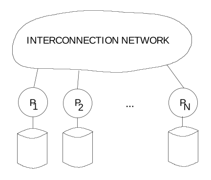
Gamma is based on the concept of a shared-nothing architecture in which processors do not share disk drives or random access memory and can only communicate with one another by sending messages through an interconnection network. Mass storage in such an architecture is generally distributed among the processors by connecting one or more disk drives to each processor.

Reasons why the shared-nothing approach has become the architecture of choice.

• There is nothing to prevent the architecture from scaling to 1000s of processors unlike shared-memory machines for which scaling beyond 30-40 processors may be impossible.
• By associating a small number of disks with each processor and distributing the tuples of each relation across the disk drives, it is possible to achieve very high aggregate I/O bandwidths without using custom disk controllers

When Gamma’s system is figuring out the best way to run a query, it uses information about how the data is divided up (partitioned). This partitioning information helps the system decide how many processors (computers) need to be involved in running the query.

• For hash partitioning: If a table (say, “X”) is divided based on a hash function applied to a certain column (like “y”), and the query asks for records where “X.y = some value,” the system can directly go to the specific processor that holds the data matching that value.
• For range partitioning: If the table is divided based on ranges of values for a column, the system can limit the query to only the processors that have data within the relevant range. For example, if “X” is partitioned such that one processor handles values from 1 to 100, and another handles values from 101 to 200, then a query asking for “X.y between 50 and 150” will involve only the processors that have data in those ranges.

Different processes in the Gamma system work together. Here’s a simplified explanation of the main types of processes and their roles:

1. Catalog Manager: Acts like a “database encyclopedia,” storing all the information about data tables and structures. It ensures that data remains consistent when multiple users access the database.

2. Query Manager: Each user gets a query manager that handles query requests. It is responsible for parsing the query, optimizing it, and generating the execution plan.

3. Scheduler Processes: When a query is executed, the scheduler coordinates the execution steps. It activates the necessary operator processes (such as scan, selection, etc.) and ensures that all steps are performed in the correct order.

4. Operator Processes: These processes carry out specific database operations, like filtering data or joining tables. To reduce the startup delay during query execution, some operator processes are pre-initialized when the system starts.

5. Other Processes:

   • Deadlock Detection Process: Detects situations where two or more processes are stuck waiting for each other to release resources.

   • Recovery Process: Manages data recovery after a system failure.

How the Gamma system executes database queries?

1. Query Parsing and Optimization: When a user submits a query, Gamma first parses it to understand what the query is asking for. Then, the system optimizes the query to find the most efficient way to execute it.
2. Query Compilation: After optimization, the query is compiled into an “operator tree“ made up of different operations (such as scan, selection, join, etc.). This tree outlines the steps and the order in which the query will be executed.
3. Single-Site vs. Multi-Site Queries: If the query only involves data on a single node (e.g., querying a small table), the system executes it directly on that node. However, if the query involves data distributed across multiple nodes (e.g., joining large tables), the system uses a “scheduler process” to coordinate the execution.
4. Scheduler Coordination: The scheduler process is responsible for activating various operator processes across the nodes, such as instructing one node to scan data while another filters it. The scheduler also manages the flow of data between these operations, ensuring they happen in the correct order.
5. Returning the Results: Once all operations are completed, the query results are collected and returned to the user. For queries embedded in a program, the results are passed back to the program that initiated the query.

Different operations (like scanning data, filtering, joining tables, etc.) are carried out in a parallel manner. Here’s a simplified explanation:

1. Operator Processes: In Gamma, each operation in a query is handled by something called an “operator process.” For example, if the query needs to scan data from a table, filter some rows, and then join with another table, there would be separate operator processes for scanning, filtering, and joining.
2. Data Flow: The data flows from one operator process to the next. For instance, the scan operator reads data from the disk and sends it to the filter operator, which then passes the filtered results to the join operator. This creates a kind of “data pipeline.”
3. Split Table: Gamma uses a “split table” to decide where the data should go next. Think of it like a routing table that directs the flow of data. For example, if the data needs to be sent to multiple nodes for parallel processing, the split table helps determine which node each piece of data should go to.
4. End of Processing: Once an operator finishes processing all its data, it closes its output streams and sends a signal to the scheduler process (which coordinates the whole query) to let it know that this part of the work is done.

In simple terms, the operator and process structure in Gamma is like an assembly line where data moves from one step (operator) to the next, with each operator performing a specific task, and the split table guiding the data flow. This setup allows the system to process data in parallel across multiple nodes, making it much faster.

Operators

Selection Operator

Data Spread Across Multiple Disks: In Gamma, data tables are split up and stored across multiple disks (this is called “declustering”). Because of this, when you want to search (select) for specific data, the system can perform the search in parallel across multiple disks.

Parallel Selection Process:

• If the search condition (predicate) matches the way the data is divided (partitioned), the system can narrow down the search to just the relevant nodes (computers with disks) that have the data. For example:
• • If the data is divided using a hash or range partitioning method based on a certain attribute (like “employee ID”), and the search is also based on that attribute (e.g., “employee ID = 123”), then the search can be directed only to the node that holds data matching that condition.
  • If the data is divided using a round-robin method (spreading data evenly across all disks) or if the search condition doesn’t match the partitioning attribute, then the system has to search on all nodes.

Performance Optimization:

• To make the search faster, Gamma uses a “read-ahead“ technique. This means that when it reads one page of data, it starts loading the next page at the same time, so that the processing of data can keep going without waiting for the next page to load.

Join Operator

Using Hash Partitioning: The join algorithms in Gamma are based on a concept called “buckets.” This means splitting the two tables to be joined into separate groups (buckets) that don’t overlap. The groups are created by applying a hash function to the join attribute (e.g., Employee ID), so that data with the same hash value ends up in the same bucket.

By partitioning the data into different buckets, each bucket contains unique data subsets, allowing parallel processing of these buckets, which speeds up the join operation. Additionally, all data with the same join attribute value is in the same bucket, making it easier to perform the join.

Gamma implements four different parallel join algorithms:

• Sort-Merge Join: Joins data by sorting and merging.
• Grace Join: A distributed hash-based join algorithm.
• Simple Hash Join: A straightforward hash-based partitioning join.
• Hybrid Hash Join: A combination of different join techniques.

Default to Hybrid Hash Join: Research showed that the Hybrid Hash Join almost always performs the best, so Gamma uses this algorithm by default.

Limitations: These hash-based join algorithms can only handle equi-joins (joins with equality conditions, like “Employee ID = Department ID”). They currently don’t support non-equi-joins (conditions like “Salary > Department Budget * 2”). To address this, Gamma is working on designing a new parallel non-equi-join algorithm.

Hybrid Hash-Join

• In the first phase, the algorithm uses a hash function to partition the inner (smaller) relation, R, into N buckets. The tuples of the first bucket are used to build an in-memory hash table while the remaining N-1 buckets are stored in temporary files. A good hash function produces just enough buckets to ensure that each bucket of tuples will be small enough to fit entirely in main memory.
• During the second phase, relation S is partitioned using the hash function from step 1. Again, the last N-1 buckets are stored in temporary files while the tuples in the first bucket are used to immediately probe the in-memory hash table built during the first phase.
• During the third phase, the algorithm joins the remaining N-1 buckets from relation R with their respective buckets from relation S.

The join is thus broken up into a series of smaller joins; each of which hopefully can be computed without experiencing join overflow. The size of the smaller relation determines the number of buckets; this calculation is independent of the size of the larger relation.

Parallel version of Hybrid Hash-Join

Partitioning into Buckets: The data from the two tables being joined is first divided into N buckets (small groups). The number of buckets is chosen so that each bucket can fit in the combined memory of the processors that are handling the join.

Storage of Buckets: Out of the N buckets, N-1 buckets are stored temporarily on disk across different disk sites, while one bucket is kept in memory for immediate processing.

Parallel Processing: A joining split table is used to decide which processor should handle each bucket, helping to divide the work across multiple processors. This means that different processors can work on different parts of the join at the same time, speeding up the process.

Overlapping Phases for Efficiency:

• When partitioning the first table (R) into buckets, Gamma simultaneously builds a hash table for the first bucket in memory at each processor.
• When partitioning the second table (S), Gamma simultaneously performs the join for the first bucket from S with the first bucket from R. This way, partitioning and joining overlap, making the process more efficient.

Adjusting the Split Table for Parallel Joining: The joining split table is updated to make sure that the data from the first bucket of both tables is sent to the right processors that will perform the join. When the remaining N-1 buckets are processed, only the routing for joining is needed.

Aggregate Operator

Parallel Calculation of Partial Results: Each processor in the Gamma system calculates the aggregate result for its own portion of the data simultaneously. For example, if the goal is to calculate a sum, each processor will first compute the sum for the data it is responsible for.

Combining Partial Results: After calculating their partial results, the processors send these results to a central process. This central process is responsible for combining all the partial results to produce the final answer.

Two-Step Computation:

• Step 1: Each processor calculates the aggregate value (e.g., sum, count) for its data partition, resulting in partial results.
• Step 2: The processors then redistribute these partial results based on the “group by” attribute. This means that the partial results for each group are collected at a single processor, where the final aggregation for that group is completed.

Update Operator

For the most part, the update operators (replace, delete, and append) are implemented using standard techniques. The only exception occurs when a replace operator modifies the partitioning attribute of a tuple. In this case, rather than writing the modified tuple back into the local fragment of the relation, the modified tuple is passed through a split table to determine which site should contain the tuple.

Concurrency Control

Gamma uses a two-phase locking strategy to manage concurrency. This means that before accessing data, a process must first acquire locks (first phase), and then release the locks after completing its operations (second phase). This ensures that multiple operations do not modify the same data at the same time, preventing conflicts.

Gamma supports two levels of lock granularity: file-level and page-level (smaller scope). There are also five lock modes:

• S (Shared) Lock: Allows multiple operations to read the data simultaneously.
• X (Exclusive) Lock: Only one operation can modify the data, while others must wait.
• IS, IX, and SIX Locks: Used to manage locking at larger scopes, such as entire files, allowing different combinations of read and write permissions.

Each node in Gamma has its own lock manager and deadlock detector to handle local data locking. The lock manager maintains a lock table and a transaction wait-for-graph, which tracks which operations are waiting for which locks.

The cost of setting a lock depends on whether there is a conflict:

• No Conflict: Takes about 100 instructions.
• With Conflict: Takes about 250 instructions because the system needs to check the wait-for-graph for deadlocks and suspend the requesting transaction using a semaphore mechanism.

Gamma uses a centralized deadlock detection algorithm to handle deadlocks across nodes:

• Periodically (initially every second), the centralized deadlock detector requests each node’s local wait-for-graph.
• If no deadlock is found, the detection interval is doubled (up to 60 seconds). If a deadlock is found, the interval is halved (down to 1 second).
• The collected graphs are combined into a global wait-for-graph. If a cycle is detected in this global graph, it indicates a deadlock.

When a deadlock is detected, the system will abort the transaction holding the fewest locks to free up resources quickly and allow other operations to proceed.

Recovery and Log

Logging Changes:

When a record in the database is updated, Gamma creates a log record that notes the change. Each log record has a unique identifier called a Log Sequence Number (LSN), which includes a node number (determined when the system is set up) and a local sequence number (which keeps increasing). These log records are used for recovery if something goes wrong.

Log Management:

• The system sends log records from query processors to Log Managers, which are separate processors that organize the logs into a single stream.
• If there are multiple Log Managers (M of them), a query processor sends its logs to one of them based on a simple formula: processor number mod M. This way, each query processor always sends its logs to the same Log Manager, making it easy to find logs later for recovery.

Writing Logs to Disk:

• Once a “page” of log records is filled, it is saved to disk.
• The Log Manager keeps a Flushed Log Table, which tracks the last log record written to disk for each node. This helps know which logs are safely stored.

Writing Data to Disk (WAL Protocol):

• Before writing any changed data (a dirty page) to disk, the system checks if the corresponding log records have already been saved.
• If the logs are saved, the data can be safely written to disk. If not, the system must first ensure the logs are written to disk before proceeding.
• To avoid waiting too long for log confirmations, the system always tries to keep a certain number of clean buffer pages (unused pages) available.

Commit and Abort Handling:

• Commit: If a transaction completes successfully, the system sends a commit message to all the relevant Log Managers.
• Abort: If a transaction fails, an abort message is sent to all processors involved, and each processor retrieves its log records to undo the changes using the ARIES algorithm, which rolls back changes in the reverse order they occurred.

Recovery Process:

• The system uses the ARIES algorithms for undoing changes, checkpointing, and restarting after a crash.
• Checkpointing helps the system know the most recent stable state, reducing the amount of work needed during recovery.

Dataflow scheduling technologies

1. Data-Driven Execution Instead of Operator Control: Gamma’s dataflow scheduling lets data automatically move between operators, forming a pipeline. Each operator acts like a step on an assembly line: when data reaches the operator, it processes the data and then passes the processed results to the next operator.
2. Reducing Coordination Overhead: Because of this dataflow design, the system does not need to frequently coordinate or synchronize the execution of each operator. This approach reduces the complexity and overhead of scheduling, especially when multiple operators are running in parallel, and avoids performance bottlenecks caused by waiting or synchronization.
3. Inherent Support for Parallelism: Dataflow scheduling is well-suited for parallel processing because data can flow between multiple operators at the same time. For example, a query can simultaneously perform scanning, joining, and aggregation across different processors. Each operator can independently process the data it receives without waiting for other operators to finish, allowing the system to efficiently utilize the computational power of multiple processors.
4. Adaptability to Dynamic Environments: During query execution, dataflow scheduling can be adjusted based on the actual system load and data characteristics. This flexibility allows the system to dynamically optimize the performance of query execution, especially for large and complex queries, by better adapting to changing query demands and system conditions.

Gamma’s unique dataflow scheduling techniques allow data to flow naturally between operators, reducing the need for direct control over operations. This significantly lowers coordination overhead in multi-processor environments, enhances the system’s parallel processing capabilities, and improves the efficiency of executing complex queries.

In Gamma’s dataflow scheduling techniques, parallelism is extensively used to improve query execution efficiency. Here’s where and how parallelism is applied:

1. Parallel Execution of Operators: Queries often involve multiple operators (e.g., scan, filter, join, aggregation). With dataflow scheduling, these operators can run in parallel:

   • Scan and Filter in Parallel: While one processor scans a data block, another processor can be filtering the data from previous blocks.

   • Parallel Joins: If a join operation involves large datasets distributed across different nodes, Gamma can perform the join operation on these different parts of the data simultaneously. The result of the join is computed in parallel across multiple processors.

2. Data Partitioning for Parallelism: The relations (data tables) are often partitioned across multiple processors in Gamma. This means that different processors can work on different partitions of the data at the same time. For example:

   • Partitioned Hash Joins: Data can be split into “buckets” based on a hash function, and different processors can handle the join for different buckets simultaneously.

   • Parallel Aggregation: When computing aggregate functions (e.g., sum or average), each processor calculates a partial result for its own partition of the data, and these partial results are later combined.

In summary, parallelism in Gamma is achieved through:

• Distributing query operators across multiple processors.
• Partitioning data so different processors work on different sections simultaneously.
• Enabling multiple stages of query execution (e.g., scanning, filtering, joining) to happen concurrently.

Questions

What is a fragment or a shard in Gamma?

A fragment or shard refers to a portion of a database relation that is horizontally partitioned across multiple disk drives.

How does a Gamma operator know where to send its stream of records?

There is a structure called split table to determine where each tuple should be sent, based on the values of tuples.

With interleaved declusttering, why not use a cluster size that includes all nodes in the system?

If an interleaved declustteing system includes all nodes, it will become more vulnerable to failures. The failure of any two nodes could make the data inaccessible. A smaller cluster will limits the risk of complete data unavailability and balance the load.

Hash-join is appropriate for processing equi-join predicates (Emp.dno = Dept.dno). How can Gamma process nonequi-join predicates (Emp.Sal > Dept.dno*1000) in a pipelined manner?

Range partitioning: Pre-partition the data based on ranges of values to reduce the search space.

Broadcast join: When the smaller relation is broadcasted to all nodes, and then each node evaluates the nonequi-join predicate in parallel.

Nested-loop join: Use a nested-loop join strategy where each tuple from one relation is compared against all tuples from the other relation.

What is the difference between Gamma, Google MapReduce, Microsoft Dryad and Apache Flink?

Will a version of Gamma using FLOW be more modular than its current design?

Yes. FLOW enables more fine-grained control over the data flow and process interactions, which could simplify the addition of new operators and functionalities. It would also make the system easier to maintain and extend, as each component could be developed and optimized independently.

Reference: https://pages.cs.wisc.edu/~dewitt/includes/paralleldb/ieee90.pdf