Greedy Dual Size (GDS) algorithm

Key Concepts:

1. Variable Size and Cost:
   • Unlike simple algorithms that treat all objects equally, GDS takes into account:
     • Size of the object (size(p)): Larger objects take up more space in memory.
     • Cost of the object (cost(p)): This can represent factors like time to retrieve the object, computational effort, or other resource usage.
2. Score H(p):
   • Each key-value pair ppp in the cache is assigned a score H(p). This score reflects the benefit of keeping the object in memory and is calculated using:
     • A global parameter L, which adjusts dynamically based on cache state.
     • The size(p) of the object.
     • The cost(p) associated with the object.
3. Eviction Strategy:
   • When the cache is full, and a new object needs to be added, GDS removes the object with the lowest score H(p). This process continues until there is enough space for the new object.

Proposition 1

L is non-decreasing over time.

• The global parameter L, which reflects the minimum priority H(p) among all key-value pairs in the KVS, will either stay the same or increase with each operation. This ensures stability and helps prioritize eviction decisions consistently.

For any key-value pair ppp in the KVS, the relationship holds:

L ≤ H(p) ≤ L + cost(p) / size(p)

• H(p), the priority of p, always lies between the global minimum L and L + cost(p) / size(p), ensuring H(p) reflects both its retrieval cost and size relative to other elements.

Intuition Behind Proposition 1:

• As L increases over time (reflecting the minimum H(p)), less recently used or less “valuable” pairs become increasingly likely to be evicted. This ensures that newer and higher-priority pairs stay in the KVS longer.

Key Insights from Proposition 1:

1. Delayed Eviction:
   • When p is requested again while in memory, its H(p) increases to L + cost(p) / size(p), delaying its eviction.
2. Impact of Cost-to-Size Ratio:
   • Pairs with higher cost(p) / size(p) stay longer in the KVS. For example, if one pair’s ratio is c times another’s, it will stay approximately c times longer.

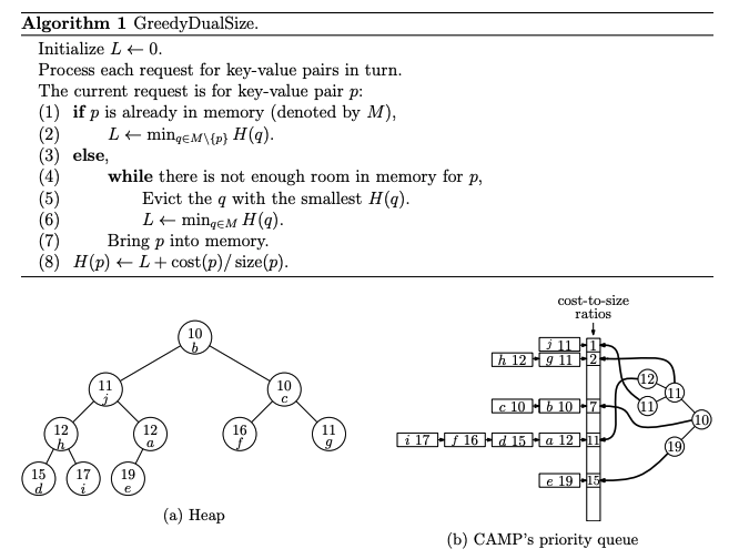
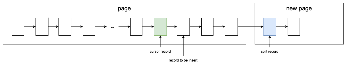
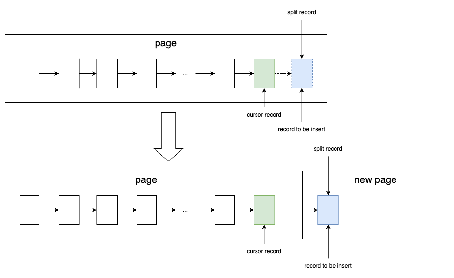
Key Points in the Diagram

1. Cost-to-Size Ratios:
   1. Key-value pairs are grouped into queues according to their cost-to-size ratio.
   2. Each queue corresponds to a specific cost-to-size ratio.
2. Grouping by Ratio:
   1. Within each queue, key-value pairs are managed using the Least Recently Used (LRU) strategy.
3. Priority Management:
   1. The priority (H-value) of a key-value pair is based on: H(p) = L + cost(p) / size(p)
      1. L: The global non-decreasing variable.
      2. cost(p) / size(p): The cost-to-size ratio of the key-value pair.
4. Efficient Eviction:
   1. CAMP maintains a heap that points to the head of each queue, storing the minimum H(p) from every queue.
   2. To identify the next key-value pair for eviction:
      1. The algorithm checks the heap to find the queue with the smallest H(p).
      2. It then evicts the key-value pair at the front of that queue (i.e., the least recently used pair in that cost-to-size group).

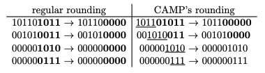
Rounding in CAMP

1. Purpose: To improve performance, CAMP reduces the number of LRU queues by grouping key-value pairs with similar cost-to-size ratios into the same queue.
2. Key Idea: Preserve the most significant bits proportional to the value’s size.

Proposition 2: Explanation of Rounding and Distinct Values

Implications

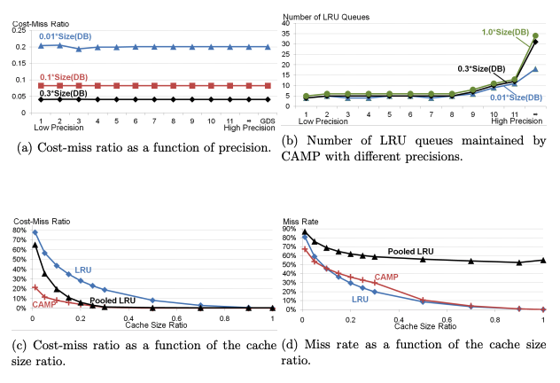
1. Trade-Off Between Precision and Efficiency:

   • A higher p preserves more precision but increases the number of distinct values (and thus computational complexity).

   • Lower p reduces the number of distinct values, making CAMP more efficient but less precise.

2. Rounding Efficiency:

   • By limiting the number of distinct values, CAMP minimizes the number of LRU queues, reducing overhead while still approximating GDS closely.

Proposition 3: Competitive Ratio of CAMP

Practical Implications

1. Precision ppp:

   • The smaller the ϵ (higher ppp), the closer CAMP approximates GDS.

   • For sufficiently large p, CAMP performs nearly as well as GDS.

2. Trade-off:

   • Higher p increases precision but also increases the number of distinct cost-to-size ratios and computational overhead.

CAMP’s Improvement Over GDS:

1. Approximation: CAMP simplifies H(p) by rounding the cost-to-size ratio, reducing the precision but making the algorithm more efficient.
2. Grouping: Key-value pairs are grouped by similar cost-to-size ratios, reducing the number of queues and simplifying priority management.
3. Tie-Breaking: CAMP uses LRU within each group to determine the eviction order, making it computationally cheaper.

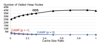
Figure 4: Heap Node Visits

This figure compares the number of heap node visits for GDS and CAMP as a function of cache size:

1. GDS:

   • Heap size equals the total number of key-value pairs in the cache.

   • Every heap update (insertion, deletion, or priority change) requires visiting O(log⁡n) nodes, where n is the number of cache entries.

   • As cache size increases, GDS’s overhead grows significantly.

2. CAMP:

   • Heap size equals the number of non-empty LRU queues, which is much smaller than the total number of cache entries.

   • Heap updates occur only when:

     • The priority of the head of an LRU queue changes.

     • A new LRU queue is created.

   • As cache size increases, the number of non-empty LRU queues remains relatively constant, resulting in fewer heap updates.

Evaluation

(a) Cost-Miss Ratio vs Precision

• 横轴：精度（Precision），从低到高。
• 纵轴：成本未命中比（Cost-Miss Ratio）。
• 结果：
  • 不同的缓存大小比（0.01、0.1 和 0.3）在较低精度下表现一致。
  • 提高精度后，成本未命中比没有显著变化。
  • 说明即使使用较低精度，CAMP 的成本未命中比也能接近 GDS（标准实现）。

(b) LRU Queues vs Precision

• 横轴：精度（Precision）。
• 纵轴：CAMP 维护的非空 LRU 队列数量。
• 结果：
  • 低精度（1-5）：CAMP 维持稳定的少量 LRU 队列（约 5 个）。
  • 高精度（>10）：队列数增加，尤其是在较大的缓存大小比（如 1.0）下。
  • 结论：
    • 在较低精度下，CAMP 能保持较低的计算开销，同时维持高效的队列管理。

(c) Cost-Miss Ratio vs Cache Size Ratio

• 横轴：缓存大小比（Cache Size Ratio），即缓存大小与 trace 文件中唯一键值对总大小的比值。
• 纵轴：成本未命中比（Cost-Miss Ratio）。
• 结果：
  • CAMP：
    • 在所有缓存大小下，成本未命中比最低。
    • 说明 CAMP 在高成本键值对管理上更具效率。
  • Pooled LRU：
    • 在较小缓存下表现稍差，但随着缓存增加，接近 CAMP。
  • LRU：
    • 成本未命中比始终最高。
  • 结论：
    • CAMP 优于 LRU 和 Pooled LRU，尤其是在小缓存下。

(d) Miss Rate vs Cache Size Ratio

• 横轴：缓存大小比（Cache Size Ratio）。
• 纵轴：未命中率（Miss Rate）。
• 结果：
  • CAMP：
    • 未命中率显著低于 LRU 和 Pooled LRU，尤其在小缓存下表现最优。
  • Pooled LRU：
    • 未命中率随着缓存增大而下降，但始终高于 CAMP。
    • 最低成本池（cheapest pool）未命中率接近 100%，次低成本池未命中率达到 65%。
  • LRU：
    • 始终高于 CAMP 和 Pooled LRU。
  • 结论：
    • CAMP 在多种缓存大小下都保持较低的未命中率，且比 Pooled LRU 更均衡。

CAMP 的适应能力：访问模式变化的分析

实验设置：

• 使用 10 个不同的 trace 文件，每个文件包含 400 万个键值对引用。
• 每个 trace 文件（如 TF1、TF2 等）中的请求在其结束后不会再被引用，模拟访问模式的突然变化。
• 访问模式具有倾斜分布（如 Zipf 分布），每个 trace 文件中的高成本对象可能在下一次访问中完全无效。

目标：

• 比较 CAMP、Pooled LRU 和 LRU 在不同缓存大小下对访问模式突变的适应能力。
• 评估三种算法在突然变化后清除旧的高成本键值对的效率，以及对总体性能（如成本未命中比和未命中率）的影响。

不同算法的行为分析

1. LRU：

   • 按最近使用排序，当新请求的总大小超过缓存大小时清除旧数据。

   • 当缓存大小比为 1 时，清除 TF1 数据的时间点对应于 TF3 开始请求的第一个键值对。

2. Pooled LRU：

   • 将键值对按成本分组，每组分配固定比例的缓存空间。

   • 高成本池占据 99% 的缓存空间，因此在每个新 trace 开始时会突然清除一批旧数据。

   • 对于缓存大小比 2/3 或更高的情况，直到 TF4（约 800 万请求后）才会清除所有 TF1 数据。

3. CAMP：

   • 对每个成本-大小比维护 LRU 队列，这些队列的大小可以动态调整。

   • 优先淘汰较低优先级的数据，但高成本数据即使来自旧 trace，也具有一定保留优先级。

   • 当新数据的总大小超过缓存时，旧 trace 的高成本数据才会被逐步清除。

图 6c：缓存比 0.25（小缓存）

1. LRU：

   • 清除最快，仅需 2.1 万次请求 即完全清除 Trace 1 的所有键值对。

   • 由于 LRU 优先淘汰最久未使用的数据，小缓存下表现最佳。

2. Pooled LRU：

   • 清除速度较慢，需要 13.1 万次请求。

   • 原因：Pooled LRU 按成本对键值对分组，高成本池占用较多缓存空间，导致清除滞后。

3. CAMP：

   • 初期清除速度比 Pooled LRU 更快，但最后完全清除所有键值对需到 TF3 结束（770 万次请求）。

   • 然而，这些未被清除的 Trace 1 数据仅占缓存的 2%，说明 CAMP 优先保留了高成本键值对。

图 6d：缓存比 0.75（大缓存）

1. LRU：

   • 同样清除最快，几乎在 Trace 2 开始时就清除掉大部分 Trace 1 的数据。

   • 说明即使缓存较大，LRU 仍然倾向淘汰旧数据。

2. Pooled LRU：

   • 清除延迟显著，需要 730 万次请求，接近 TF3 结束。

   • 原因：高成本池占用过多缓存空间，延迟清除低成本和无用数据。

3. CAMP：

   • 大部分 Trace 1 数据在较早阶段被淘汰，仅保留少量最昂贵的键值对（占缓存比小于 0.6%）。

   • 即使在 4000 万次请求后，这些高成本键值对仍在缓存中，但对整体缓存利用影响极小。

针对不同大小但成本相同的键值对，CAMP 优先保留较小的键值对，从而降低未命中率和成本未命中比。

针对相同大小但成本不同的键值对，CAMP 优先保留高成本键值对，在成本未命中比上显著优于其他算法。

与其他算法的对比：

• LRU：适用于简单场景，但无法处理成本差异。

• Pooled LRU：小缓存情况下表现不错，但静态分区策略限制了其大缓存场景的效率。

CAMP 的适应性：在处理多样化的成本分布时，通过动态调整和四舍五入策略，CAMP 在复杂负载下表现出更高的灵活性和效率。

Questions

What is the time complexity of LRU to select a victim?

O(1) because the least recently used item is always at the tail of the list.

What is the time complexity of CAMP to select a victim?

O(logk) CAMP identifies the key-value pair with the smallest priority from the heap, deletes it and then heapifies.

Why does CAMP do rounding using the high order bits?

• CAMP rounds cost-to-size ratios to reduce the number of distinct ratios (or LRU queues).
• High-order bits are retained because they represent the most significant portion of the value, ensuring that approximate prioritization is maintained.

How does BG generate social networking actions that are always valid?

Pre-Validation of Actions:

• Before generating an action, BG checks the current state of the database to ensure the action is valid. For instance:
  • A friend request is only generated if the two users are not already friends or in a “pending” relationship.
  • A comment can only be posted on a resource if the resource exists.

Avoiding Concurrent Modifications:

• BG prevents multiple threads from concurrently modifying the same user’s state.

How does BG scale to a large number of nodes?

BG employs a shared-nothing architecture with the following mechanisms to scale effectively:

1. Partitioning Members and Resources:

   • BGCoord partitions the database into logical fragments, each containing a unique subset of members, their resources, and relationships.

   • These fragments are assigned to individual BGClients.

2. Multiple BGClients:

   • Each BGClient operates independently, generating workloads for its assigned logical fragment.

   • By running multiple BGClients in parallel across different nodes, BG can scale horizontally to handle millions of requests.

3. D-Zipfian Distribution:

   • To ensure realistic and scalable workloads, BG uses a decentralized Zipfian distribution (D-Zipfian) that dynamically assigns requests to BGClients based on node performance.

   • Faster nodes receive a larger share of the logical fragments, ensuring even workload distribution.

4. Concurrency Control:

   • BG prevents simultaneous threads from issuing actions for the same user, maintaining the integrity of modeled user interactions and avoiding resource contention.

True or False: BG quantifies the amount of unpredictable data produced by a data store?

True.

This is achieved through:

• Validation Phase:
  • BG uses read and write log records to detect instances where a read operation observes a value outside the acceptable range, classifying it as “unpredictable data.”
• Metrics Collection:
  • The percentage of requests that observe unpredictable data (τ) is a key metric used to evaluate the data store’s consistency.

How is BG’s SoAR different than its Socialites rating?

SoAR (Social Action Rating): Represents the maximum throughput (actions per second) a data store can achieve while meeting a given SLA.

Socialites Rating: Represents the maximum number of concurrent threads (users) a data store can support while meeting the SLA.

Reference: https://citeseerx.ist.psu.edu/document?repid=rep1&type=pdf&doi=d6f9678772a09ca29101f5efce583960ecf53745

索引是一种可以帮助 MySQL 高效获取数据的数据结构，也是有序结构。

优点

• 提高数据检索效率，降低数据库 I/O 成本。
• 通过索引列对数据进行排序，降低数据排序成本，降低 CPU 的消耗。

缺点

• 占用空间。
• 降低了更新表的效率，如 INSERT、UPDATE、DELETE。

因此，若索引太多，应用程序的性能可能会受到影响。而索引太少，对查询性能又会产生影响。要找到一个合适的平衡点，这对应用程序的性能至关重要。

索引结构

MySQL 索引是在引擎层实现的，不同的存储引擎支持不同的索引结构。

InnoDB 索引分类

根据索引存储形式，可分为以下两种：

InnoDB 支持以下索引：

• B+ 树索引
• 全文索引
• 自适应 Hash 索引

B+ 树索引就是传统意义上的索引，这是目前关系型数据库系统中查找最为高效且被认为有效的索引。B+ 树索引的构造类似于二叉树，根据键值（Key Value）快速找到数据。B+ 树索引能找到的只是被查找数据所在的页。然后数据库通过把页读入到内存，再在内存中进行查找，最后得到要查找的数据。

整体流程：

B+ 树 Root => B+ 树索引节点 => B+ 树叶子节点 => Page Directory 中的一个 Slot => 目标行数据。

InnoDB 存储引擎支持的哈希索引是自适应的，InnoDB 存储引擎会根据表的使用情况自动为表生成哈希索引，不能人为干预是否在一张表中生成哈希索引。

InnoDB 的主键使用的是聚簇索引，而 MyISAM 中，不管是主键索引还是二级索引使用的都是非聚簇索引。

InnoDB 中的全表扫描会顺序读取聚集索引上的数据页（即叶子节点），等价于按主键顺序逐行扫描表中所有行。

全表扫描

在 InnoDB 中，一条简单的 SELECT * FROM A 在执行时会经过以下几层，才能把表 A 中的每一行读出来。下面分段结合关键源码，逐步说明一个典型的全表扫描流程。

一、Handler 接口：ha_rnd_next 循环读取

TableScanIterator::Read() 中：

1
2
3
4
5
6
7

while ((tmp = table()->file->ha_rnd_next(m_record))) {

  if (tmp == HA_ERR_RECORD_DELETED && !thd()->killed) continue;

  return HandleError(tmp);

}

• ha_rnd_next(m_record)：MySQL 存储引擎统一接口，每次调用读一行到 m_record。

• 跳过 DELETED：MyISAM 在并发删时会返回 HA_ERR_RECORD_DELETED，此处跳过。

• 返回码：0 表示成功取到一行；非 0 则调用 HandleError(tmp) 终止扫描。

对于 InnoDB，ha_rnd_next 内部实现为：

1
2
3
4
5
6
7
8
9
10
11
12
13

int handler::ha_rnd_next(uchar *buf) {

  MYSQL_TABLE_IO_WAIT(..., { result = rnd_next(buf); })

    if (!result && m_update_generated_read_fields)

      update_generated_read_fields(buf, table);

  table->set_row_status_from_handler(result);

  return result;

}

二、InnoDB 读取流程：rnd_next → general_fetch → row_search_mvcc

rnd_next(buf) 中的核心调用如下：

1
2
3
4
5
6
7
8
9
10
11
12
13

if (m_start_of_scan) {

  error = index_first(buf);

  m_start_of_scan = false;

} else {

  error = general_fetch(buf, ROW_SEL_NEXT, 0);

}

return error;

• 首次扫描 调用 index_first(buf) 定位到最左叶节点的第一条记录；
• 后续扫描 一律调用 general_fetch。

general_fetch(buf, ROW_SEL_NEXT, 0) 中的核心调用如下：

1
2
3
4
5
6
7

if (!intrinsic) // 普通表

  ret = row_search_mvcc(buf, PAGE_CUR_UNSUPP, m_prebuilt, 0, ROW_SEL_NEXT);

// ...

// 再把 dberr_t 转成 MySQL 错误码返回给 rnd_next

row_search_mvcc

row_search_mvcc 中的核心调用如下：

• 首次 (direction == 0)：构造或恢复一个 B-树游标 pcur，调用 pcur->open_no_init()（或 open_at_side）从根节点一路走到左最叶，定位第一条记录。
• 后续 (direction == ROW_SEL_NEXT)：直接在叶节点上调用 pcur->move_to_next(&mtr)，利用叶节点之间的双向链表遍历下一条记录，无需再从根节点重查。
• 循环过滤（rec_loop）：
  • 跳过 infimum/supremum 伪记录，检查页内偏移合法性；
  • MVCC 版本检查：如果当前版本不可见，调用 undo log 回溯到可见版本；
  • 删除标记：跳过 delete-marked；
  • 索引条件下推（此例没有 WHERE，相当于 match_mode == 0，所有行都通过）；
  • 转换格式：调用 row_sel_store_mysql_rec(buf, …) 将内部二进制行转成 MySQL 客户端格式；
  • 预取缓存：若启用缓存则放入队列，否则直接写入 buf 并 return DB_SUCCESS。
• 退出：当 move_to_next 返回 false（无更多记录），函数最终返回 DB_END_OF_INDEX 或 DB_RECORD_NOT_FOUND，上层映射为 HA_ERR_END_OF_FILE。

在 row_search_mvcc 的整个执行过程中，游标（pcur）的状态会在多处被保存和恢复，其核心目的有两个：

1. 跨页扫描时保持定位：当 B- 树叶节点遍历到一页的末尾，需要切换到下一页时，InnoDB 会提交当前 mini-transaction（mtr_commit(&mtr)）并重新开启一个新的 mini-transaction（mtr_start(&mtr)）。提交会释放当前页面的读锁（latch），以避免死锁或锁的过度持有。但一旦释放，就无法再在页内继续定位，于是必须在释放前存储当前位置，切换后再恢复，才能从下一个页的正确位置继续扫描。
2. 出现锁等待或错误时的回退：如果在给某条记录加锁过程中遇到锁等待（DB_LOCK_WAIT）或其他可重试的错误，函数会
   • 在释放 mini-transaction、让出 latch 之前存储游标位置，
   • 等待锁或错误解决后，再恢复游标，继续当前记录或下一条记录的扫描，保证最终不会漏读也不重复读。

完整调用链一览

1
2
3
4
5
6
7
8
9
10

mysql_select()
 └─ join_read_table() / read_table_rows()
   	└─ handler::ha_rnd_next(buf)
       └─ rnd_next(buf)
          ├─ index_first(buf)     // 第一次，从根到左叶
          └─ general_fetch(buf,…)  // 后续，调用 row_search_mvcc
         		 └─ row_search_mvcc(buf,…)
                ├─ pcur->open_no_init()   // 定位（首次）
                ├─ pcur->move_to_next()   // 遍历（后续）
                └─ row_sel_store_mysql_rec // 转换格式

此外，整个过程主要涉及两类锁：

元数据锁（MDL，Metadata Lock）

• MDL_SHARED_READ：在执行任何 SELECT 时，MySQL 都会在打开表的时候对表结构加一个元数据读锁，类型叫 MDL_SHARED_READ。
  • 作用：保证在查询进行时，表定义（DDL）不会被改动（比如 ALTER TABLE）。
  • 持续时间：从打开表到查询结束（close_tables()）为止。

InnoDB 内部的短期页锁（Latch）与 MVCC

• 页锁（Page Latch）：为了从缓冲池安全地读取 B+ 树节点和行记录，InnoDB 在内存页上会拿短期的读或写 latch（互斥锁），确保数据页在读取/解码时不被并发修改。
  • 这不是 SQL 层面的锁，你在 SHOW ENGINE INNODB STATUS 能看到它们，但在 SHOW OPEN TABLES 或 INFORMATION_SCHEMA.INNODB_TRX 中看不到。
• MVCC 版本控制：默认一致性读不会向行上加记录锁或间隙锁；它通过读视图加上 undo log 回溯来返回符合快照的行版本。
  • 不产生任何行锁，也不会阻塞并发的 UPDATE/DELETE。
  • 只有在遇到刚提交的、版本不可见的行时，InnoDB 会临时读取 undo log 中的旧版本，但这也是通过读取 undo 区块，不会在真正的索引上留下锁。

而且需要注意的是，整个流程中的数据是被一条条地读取并存储到 Record Buffer 中的，这就是 Valcano 风格的 pull-based Iteration Model 的体现。

并行化增强

我们可以对全表扫描进行并行化增强。因为 MySQL 在 InnoDB 层引入了并行扫描功能，用于加速需要全表扫描的操作，该功能自 8.0.14 版本开始支持，通过将 B+ 树划分为多个子树并由多个工作线程并行扫描来实现。要启用并行全表扫描，只需将会话级或全局变量 innodb_parallel_read_threads 设置为大于 1 的值，MySQL 会根据该值和实际子树数量来决定并行线程数。

配置参数 innodb_parallel_read_threads：

• 作用：控制 InnoDB 层并行扫描主键索引时的线程数，仅支持主键（聚簇索引）扫描，不支持二级索引扫描。
• 默认值：默认值为可用逻辑处理器数除以 8，至少 4；MySQL 8.4 之前始终为 4。
• 范围：1 至 256，总线程数上限为 256（跨所有会话）; 达到上限后会话会回退到单线程扫描。

动态修改：支持会话级和全局级动态设置，例如：

1
2

SET GLOBAL innodb_parallel_read_threads = 16;
SET SESSION innodb_parallel_read_threads = 8;

然后执行需要全表扫描的 SQL 即可利用并行扫描。

其他相关参数

• innodb_ddl_threads：控制并行创建二级索引或重建表时的排序和 B+ 树构建线程数。
• innodb_ddl_buffer_size：并行 DDL 操作的排序缓冲区总大小，应配合 innodb_parallel_read_threads 一同调优。

并行扫描原理

MySQL 并行查询实际上是对 B+ 树的并行扫描。核心流程如下：

1. 调用扫描接口：用户线程执行如 SELECT COUNT(*) 等语句后，进入 InnoDB 并行扫描逻辑，从 row_scan_index_for_mysql 接口开始分发任务。
2. 预分片（coarse-grained sharding）：用户线程先对整个聚簇索引做粗粒度分片，将每个子树（Range），由 [start, end) 两个游标标记，放入任务队列。其中分片的步骤如下：
   1. 用户线程在预分片期间对整个索引加 INDEX S 锁，并对根页加 ROOT PAGE S 锁，确保树在分片时不会发生页分裂或新增子树。
   2. 根页每条记录都包含一个指向子树的指针。用户线程依次读取这些指针，对应第 i 条指针即第 i 个子树。
   3. 对于每个指针，沿 B+ 树从该指针所在页向下定位到最左叶记录。
   4. 在遍历过程中，对每个经过的页加 S 锁，定位完成后创建一个 Iter，其中包含原始记录指针 m_rec 和持久化游标 m_pcur，用于后续线程快速定位。
3. 创建工作线程：根据 innodb_parallel_read_threads 值启动相应数量的工作线程，然后等待所有工作线程完成。
4. 工作线程取任务：每个工作线程从队列中取出一个 Range，如粒度过大（分片数 ＞ 线程数）则再基于该 RANGE 的键值范围按同样方式二次切分，然后依次扫描该范围内的记录，通过内部函数 row_search_mvcc 获取每条记录并执行回调（如计数或检查）。
5. 结果汇总：各线程扫描完毕后，用户线程收集各子树的统计结果或校验结果，并返回给 SERVER 层。

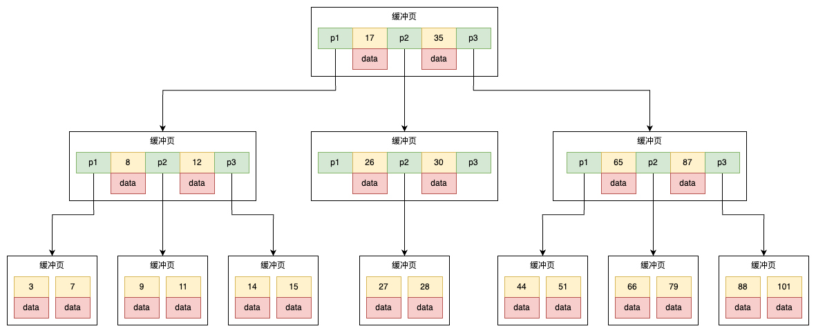
分片（Sharding）机制

并行扫描将 B+ 树划分为多个子树，每个子树对应一个 RANGE 结构体：

1
2
3
4

struct RANGE {
 Iter start; // 子树起始记录位置
 Iter end;  // 子树结束记录位置（右开区间）
};

其中 Iter 包含了记录指针和 B+ 树游标，用于定位扫描边界。工作线程可对粒度过大的 Range 再次细分，以提高负载均衡。

Iter 的结构如下：

1
2
3
4
5
6
7
8
9
10
11
12
13
14
15
16
17
18

/** Boundary of the range to scan. */
struct Iter {
 /** Destructor. */
 ~Iter();
 /** Heap used to allocate m_rec, m_tuple and m_pcur. */
 mem_heap_t *m_heap{};   // 分配迭代所需内存（记录副本、tuple、游标等）
 /** m_rec column offsets. */
 const ulint *m_offsets{}; // 原始记录中各列的偏移数组
 /** Start scanning from this key. Raw data of the row. */
 const rec_t *m_rec{};   // 指向边界记录的原始数据
 /**
  * Tuple representation inside m_rec,
  * for two Iter instances in a range m_tuple will be [first->m_tuple, second->m_tuple).
  */
 const dtuple_t *m_tuple{}; // m_rec 对应的解析后 tuple，方便按列访问
 /** Persistent cursor. */
 btr_pcur_t *m_pcur{};   // 用于快速定位 m_rec 所在页的 B+ 树游标
};

字段说明

1. m_heap：用于在堆上分配和管理该 Iter 所需的临时内存，包括存放记录副本、tuple 结构和游标状态等。
2. m_offsets：指向一组 ulint，用于记录 m_rec 中每列在页面上的偏移位置，以便快速定位列值。
3. m_rec：原始记录指针（raw record），标记分片边界的具体行数据。
4. m_tuple：m_rec 的逻辑封装（dtuple_t），两端 Iter 的 m_tuple 共同定义了扫描区间；扫描时常直接基于 m_tuple 进行比较和移动。
5. m_pcur：持久化游标（btr_pcur_t*），用于记录定位 m_rec 所在页面和行号，后续扫描可通过该游标快速恢复上次位置，而无需从根节点重定位。

支持的语句类型

目前，InnoDB 并行扫描支持以下全表操作场景：

• SELECT COUNT(*) FROM table1; 完整扫描主键索引并行计数。
• CHECK TABLE table1; 第二次扫描主键索引时可并行校验。
• CREATE INDEX … ON table1 / ALTER TABLE … ADD INDEX … 扫描和排序阶段支持并行，B+ 树构建阶段仍为单线程。
• ALTER TABLE … ENGINE=InnoDB / OPTIMIZE TABLE 重建表阶段扫描主键索引不并行，排序和索引构建支持并行。

限制与注意事项

• 并行扫描仅适用于主键索引，不支持二级索引扫描或包含虚拟列、全文索引、空间索引的表。
• 并行线程读取的数据页会被放到缓冲池 LRU 链表尾部，避免在扫描时占用过多热页。
• 当并行线程数超过子树数量时，实际使用的线程数取两者中的最小值。

B+ 树索引

B+ 树是为磁盘或其他直接存取辅助设备设计的一种自平衡的多路查找树。在 B+ 树中，所有记录节点都是按键值的大小顺序放在同一层的叶子节点上，由各叶子节点指针进行连接。

B+ 树的非叶子节点只存储键值，不存储数据，而叶子节点存储了所有的数据，并且构成了一个有序双向链表。因此，范围查询时就可以直接通过叶子节点间的指针顺序访问整个查询范围内的所有记录，而无需对树进行多次遍历。

在B+ 树的实现中，节点的大小往往被设计为与磁盘页大小相同（或者是其整数倍）。相比于 B 树（非叶子节点中存储指针和数据），B+ 树的非叶子节点能够存储更多的指针，提升索引查找的效率并且减少磁盘 I/O 次数，因为每次从磁盘中加载的节点携带了更多的指针信息。

以下是 B-Tree 的结构（绿色代表子节点的地址，黄色代表记录的主键，红色代表单条记录中除主键外的数据，之后的图也是如此）：

B-Tree可视化：B-Tree Visualization

以下是 B+ 树的结构：

B+ 树可视化：B+ Tree Visualization

也就是说，MySQL 索引数据结构在经典 B-Tree 的基础上，增加了一个指向相邻左右叶子节点的链表指针，形成了双向循环链表，这样可以方便范围查询和反向遍历。

如果需要在 B+树中从大值向小值进行范围查询，可以按以下步骤操作：

• 定位到最右侧节点：首先，找到包含最大值的叶子节点。这通常通过从根节点开始向右遍历树的方式实现。
• 反向遍历：一旦定位到了最右侧的叶子节点，可以利用叶节点间的双向链表向左遍历。

为什么Mongodb索引用B树，而MySQL用B+树?：在关系型数据库中，遍历操作比较常见，因此采用 B+ 树作为索引比较合适。而在非关系型数据库中，单一查询比较常见，因此采用 B 树作为索引比较合适。

B+ 树对于 B 树的优势：

1. 更高的查询效率： B+ 树叶子节点的双向链表使得范围查询时无需从根节点开始进行多次索引查询，只需顺序遍历双向链表即可。
2. 更高的空间利用率：B+ 树非叶子节点只存储指针，使得单个节点能够存储更多的指针只指向子节点，且单次磁盘 I/O 读取更多信息，减少 I/O 读取次数。
3. 更稳定的查询效率：B+ 树叶子节点深度相同，数据查询路径长度相同。

B+ 树对于二叉树的优势：

1. B+ 树的每个节点可以有 m 个子节点，而红黑树和二叉平衡树都只有 2 个。
2. 普通二叉树存在退化的情况，如果它退化成链表，就相当于全表扫描。
3. 读取数据的时候，是从磁盘先读到内存。平衡二叉树的每个节点只存储一个键值和数据，而 B+ 树可以存储更多的节点数据，树的高度也会降低，因此读取磁盘的次数就会下降，查询效率就快。

为什么 InnoDB 存储引擎选择使用 B+Tree 索引结构？

1. 相比于二叉树（顺序插入数据行的情况下会退化成链表），B+Tree 更平衡，层级更少，搜索效率高。
2. 就B-Tree（或 BST）而言，无论叶子节点还是非叶子节点都会保留数据，这样导致一页中存储的键减少，指针也减少了，要保存大量数据，只能增加树的高度，导致性能降低。
3. 相比于 Hash 索引，B+Tree 支持范围匹配及排序操作。

一棵 B+ 树能存储多少数据？

假如我们的主键 ID 是 bigint 类型，长度为 8 个字节。指针大小在 InnoDB 源码中设置为 6 字节，这样一共 14 字节。所以非叶子节点(一页)可以存储 $16384/14=1170$ 个这样的单元(键值+指针)。

一个指针指向一个存放记录的页，一页可以放 16 条数据，树深度为 2 的时候，可以存放 $1170*16=18720$ 条数据。

同理，树深度为 3 的时候，可以存储的数据为 $1170117016=21902400$ 条记录。

理论上，在 InnoDB 存储引擎中，B+树的高度一般为 2-4 层，就可以满足千万级数据的存储。查找数据的时候，一次页的查找代表一次 IO，当我们通过主键索引查询的时候，最多只需要 2-4 次 IO 就可以了。

B+ 树的插入操作

B+ 树的插入必须保证插入后叶子节点中的记录依然排序，同时需要考虑插入到 B+ 树的三种情况，每种情况都可能会导致不同的插入算法。具体如下：

叶子节点未满，索引节点未满：直接将记录插入到目标叶子节点的合适位置（保持有序）。

叶子节点已满，索引节点未满：

• 拆分叶子节点为左右两个节点。
• 将中间键值提升为分隔键，插入到父级索引页。
• 原叶子节点中：
  • 小于中间键值的记录 → 左侧新页；
  • 大于等于中间键值的记录 → 右侧新页。

叶子节点和索引节点都已满：

• 拆分叶子节点（Leaf Page）：

  • 小于中间键值的记录 → 左页；
  • 大于等于中间键值的记录 → 右页；

• 将中间键值提升为分隔键，插入到父级索引页。

• 由于父级索引页也已满，继续处理其溢出：

  • 拆分 Index Page：
    • 小于中间索引值的记录 → 左侧索引页；
    • 大于中间索引值的记录 → 右侧索引页；
  • 将新的中间索引项继续提升到上一层索引页中。

• 若上一层索引页仍满，则继续递归，直到根节点；若根节点也满，最终会导致根节点分裂，树高度增加。

因此，不管怎么变化，B+ 树总是会保持平衡。但是为了保持平衡，对于新插入的键值可能需要做大量的拆分页操作。因为 B+ 树结构主要用于磁盘，页的拆分意味着磁盘的操作，所以应当在可能的情况下尽量减少页的拆分操作。因此，B+ 树同样提供了类似于平衡二叉树的旋转功能。

旋转发生在叶子页（Leaf Page）已经满，但其左右兄弟节点没有满的情况下。这时 B+ 树并不会急于做拆分页的操作，而是将记录移到所在页的兄弟节点上。在通常情况下，会首先检查左兄弟以执行旋转操作。在下面的例子中：若插入键值 70，B+ 树并不会立即拆分叶子节点，而是先做旋转操作。

我们可以看到，旋转操作使得 B+ 树减少了一次页的拆分操作，同时这棵 B+ 树的高度依然为 2。

B+ 树的删除操作

B+ 树使用填充因子（fill factor）来控制树的删除变化，50% 是填充因子可设的最小值。B+ 树的删除操作同样必须保证删除后叶子节点中的记录依然排序。与插入一样，B+ 树的删除操作同样需要考虑三种情况，根据填充因子的变化来衡量是否需要进行节点合并或旋转操作。

对于第一种情况的后半部分的解释：

在以下 B+ 树中（这里省去叶节点之间的指针），我们删除键值为 25 的记录，因为该值也是 Index Page 中的值，所以在删除之后，需要将 25 的右兄弟节点的 28 更新到 Index Page 中。

以下是删除之后的 B+ 树。

这时，如果删除 Leaf Page 中键值为 60 的记录，那么 Fill Factor 小于 50%，需要做合并操作；同样，在删除 Index Page 中相关记录后，需要做 Index Page 的合并操作。结果如下：

注意：页面合并时，首先尝试与左侧直接相邻的兄弟页合并；仅在左侧不符合条件时，才会检查右侧兄弟页。如果左右两侧都没有足够的空间容纳当前页的所有记录，合并操作将不会执行，页面将保持“半空”状态，直到后续操作（如父节点合并或树高度调整）触发新的重组逻辑。合并成功后，还需在父节点中删除对应的指针条目，并在必要时向上递归合并或降高。

聚集索引

数据库中的 B+ 树索引可以分为聚集索引（clustered index）和辅助索引（secondary index）。但是无论是聚集索引还是辅助索引，其内部结构都是 B+ 树，即高度平衡的，且叶子节点存放所有的数据。聚集索引与辅助索引的不同之处在于：叶子节点存放的是否是一整行的信息。

之前已经介绍过，InnoDB 存储引擎表是索引组织表，即表中数据按照主键顺序存放。而聚集索引就是按照每张表的主键构造一棵 B+ 树，同时叶子子节点中存放的即为整张表的行记录数据，也将聚集索引的叶子节点称为数据页。聚集索引的这个特性决定了索引组织表中数据也是索引的一部分。同 B+ 树数据结构一样，每个数据页都通过一个双向链表来进行链接。

由于实际的数据页只能按照一棵 B+ 树进行排序，因此每张表只能拥有一个聚集索引。在多数情况下，查询优化器倾向于采用聚集索引。因为聚集索引能够在 B+ 树索引的叶子节点上直接找到数据。此外，由于定义了数据的逻辑顺序，聚集索引能够特别快速地访问针对范围值的查询。查询优化器能够快速发现某一段范围的数据页需要扫描。

例如：

1
2
3
4
5
6
7
8
9
10
11
12

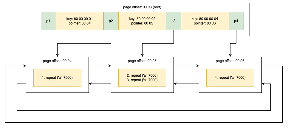
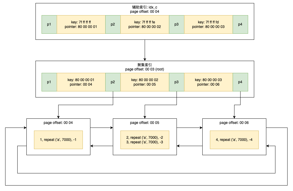
CREATE TABLE t (
 a INT NOT NULL,
 b VARCHAR(8000),
 c INT NOT NULL,
 PRIMARY KEY (a),
 KEY idx_c (c)
) ENGINE=InnoDB;

INSERT INTO t SELECT 1, REPEAT('a', 7000), -1;
INSERT INTO t SELECT 2, REPEAT('a', 7000), -2;
INSERT INTO t SELECT 3, REPEAT('a', 7000), -3;
INSERT INTO t SELECT 4, REPEAT('a', 7000), -4;

我们可以发现数据页上存放的是完整的每行记录，而在非数据页的索引页中，存放的仅仅是键值及指向数据页的偏移量，而不是一个完整的行记录。具体结构如下：

许多资料会说：聚集索引按照顺序物理地存储数据。但是试想一下，如果聚集索引必须按照特定顺序存放物理记录，则维护成本显得非常之高。所以，聚集索引的存储并不是物理上连续的，而是逻辑上连续的。这其中有两点：

1. 前面说过的页通过双向链表链接，页按照主键的顺序排列；
2. 每个页中的记录也是通过双向链表进行维护的，物理存储上可以不按主键存放。

说白了，就是在物理存储时，不同页和页内记录的数据块可以散布在数据文件各处，通过上述链表结构保证逻辑遍历顺序，从而大幅降低维护开销。

聚集索引的另一个好处是，它对于主键的排序查找和范围查找速度非常快。叶子节点的数据就是用户所要查询的数据。

还有就是范围查询（range query），即如果要查找主键某一范围内的数据，通过叶子节点的上层中间节点就可以得到页的范围，之后直接读取数据页即可。

此外，聚集索引存在如下选取规则：

• 如果存在主键，主键索引就是聚集索引。
• 如果不存在主键，将使用第一个遇到的唯一索引作为聚集索引。
• 如果既没有主键也没有合适的唯一索引，则自动生成一个以单调递增的 row ID 作为键的隐藏聚集索引。

辅助索引

对于辅助索引（Secondary Index，也称非聚集索引），叶子节点并不包含行记录的全部数据。也就是说，叶子节点除了包含键值以外，每个叶子节点中的索引行中还包含了一个书签。该书签用来告诉 InnoDB 存储引擎哪里可以找到与该索引行对应的行数据。由于 InnoDB 存储引擎表是索引组织表，因此辅助索引的书签就是相应行数据在聚集索引中的聚集索引键。

辅助索引的存在并不影响数据在聚集索引中的组织，因此每张表上可以有多个辅助索引。当通过辅助索引来寻找数据时，InnoDB 存储引擎会：

1. 遍历辅助索引树，到达叶子节点后获得对应行的聚集索引键；
2. 再通过聚集索引树查找该主键，定位到完整的行记录所在的数据页。

举例来说，如果辅助索引树的高度为 3，则需要 3 次查找才能找到指定的主键；若聚集索引树的高度也为 3，则还需要额外 3 次查找才能在聚集索引中定位到完整行的数据页。因此，总共需要 6 次逻辑 I/O 访问，才能得到最终的数据页。

示例：

在之前的表 t 上新增一列 c，并对列 c 创建聚集索引：

1
2
3
4
5
6
7
8
9
10
11
12

mysql> ALTER TABLE t
  -> ADD c INT NOT NULL;
Query OK, 4 rows affected (0.24 sec)
Records: 4 Duplicates: 0 Warnings: 0

mysql> UPDATE t SET c = 0 - a;
Query OK, 4 rows affected (0.04 sec)
Rows matched: 4 Changed: 4 Warnings: 0

mysql> ALTER TABLE t ADD KEY idx_c (c);
Query OK, 4 rows affected (0.28 sec)
Records: 4 Duplicates: 0 Warnings: 0

更改之后的索引结构如下：

上图显示了表 t 中辅助索引 idx_c 和聚集索引的关系。可以看到辅助索引的叶子节点中包含了列 c 的值和主键的值。因为这里的键值为负值，所以会发现以 7f ff ff ff 的方式进行内部存储。7（0111）最高位为 0，代表负值，实际的值应该取反后加 1，即得 -1。

B+ 树索引的分裂

之前介绍的 B+ 树分裂是最为简单的一种情况，这和数据库中 B+ 树索引的实际情况可能略有不同，因为并未涉及并发，而这才是 B+ 树索引实现中最为困难的部分。

B+ 树索引页的分裂并不总是从页的中间记录开始，这样可能会导致页空间的浪费。例如下面的记录：

1

1, 2, 3, 4, 5, 6, 7, 8, 9

插入是根据自增顺序进行的，若此时插入第 10 条记录后需要进行页的分裂操作，那么根据之前介绍的分裂方法，会将记录 5 作为分裂点记录，分裂后得到下面两个页：

Page 1: 1, 2, 3, 4；

Page 2: 5, 6, 7, 8, 9, 10。

由于插入是顺序的，P1 这个页将不会再有新记录被插入，从而导致空间浪费；而 P2 又会再次进行分裂。

InnoDB 存储引擎的 Page Header 中有以下几个部分用来保存在页中记录插入的顺序信息：

• PAGE_LAST_INSERT
• PAGE_DIRECTION
• PAGE_N_DIRECTION

通过这些信息，InnoDB 存储引擎可以决定是向左还是向右进行分裂，同时决定将分裂点记录为哪一个。若插入是随机的，则取页中的中间记录作为分裂点记录，这和之前介绍的相同。若往同一方向进行插入的记录数量为 5，并且目前已定位（cursor）到的记录（该记录为待插入记录的前一条记录）之后还有 3 条记录，则分裂点记录为定位到的记录后的第三条记录；否则，分裂点记录就是待插入的记录。

示例：

下面来看一个向右分裂的例子，并且定位到的记录之后还有 3 条记录，则分裂点记录如下：

分裂后的结果如下：

接着是分裂点就为插入记录本身：

B+ 树的管理

索引管理

索引的创建和删除可以通过两种方法，一种是 ALTER TABLE，另一种是 CREATE/DROP INDEX。通过 ALTER TABLE 创建索引的语法为：

1
2
3
4
5
6

ALTER TABLE tbl_name
ADD [INDEX|KEY] [index_name]
[index_type] (index_col_name, ...) [index_option] ...

ALTER TABLE tbl_name
DROP PRIMARY KEY | DROP {INDEX|KEY} index_name

CREATE/DROP INDEX 的语法同样很简单：

1
2
3
4

CREATE [UNIQUE] INDEX index_name
[index_type] ON tbl_name (index_col_name, ...)

DROP INDEX index_name ON tbl_name

用户可以设置对整个列的数据进行索引，也可以只索引一列的开头部分数据，如前面创建的表 t，列 b 为 varchar(8000)，但是用户可以只索引前 100 个字段，如：

1
2
3
4

mysql> ALTER TABLE t
  -> ADD KEY idx_b (b(100));
Query OK, 4 rows affected (0.32 sec)
Records: 4 Duplicates: 0 Warnings: 0

若用户想要查看表中索引的信息，可以使用命令 SHOW INDEX。我们以主键列为例，结果如下：

1
2
3
4
5
6
7
8
9
10
11
12
13
14
15

mysql> SHOW INDEX FROM t\G;
*************************** 1. row ***************************
    Table: t
    Non_unique: 0
    Key_name: PRIMARY
    Seq_in_index: 1
    Column_name: a
    Collation: A
    Cardinality: 2
    Sub_part: NULL
    Packed: NULL
    Null: 
    Index_type: BTREE
    Comment: 
…

以上结果中每列的含义如下：

Table：索引所在的表名。

Non_unique：非唯一的索引，可以看到 primary key 是 0，因为必须是唯一的。

Key_name：索引的名字，用户可以通过这个名字来执行 DROP INDEX。

Seq_in_index：索引中该列的位置，如果看联合索引 idx_a_c 就比较直观了。

Column_name：索引列的名称。

Collation：列以什么方式存储在索引中。可以是 A 或 NULL。B+ 树索引总是 A，即排序的。如果使用了 Heap 存储引擎，并且建立了 Hash 索引，这里就会显示 NULL 了。因为 Hash 根据 Hash 桶存放索引数据，而不是对数据进行排序。

Cardinality：非常关键的值，表示索引中唯一值的数目的估计值。Cardinality 表的行数应尽可能接近 1，如果非常小，那么用户需要考虑是否可以删除此索引。

Sub_part：是否是列的部分被索引。如果看到 idx_b 这个索引，这里显示 100，表示只对 b 列的前 100 字符进行索引。如果索引整个列，则该字段为 NULL。

Packed：关键字如何被压缩。如果没有被压缩，则为 NULL。

Null：是否索引的列含有 NULL 值。可以看到 idx_b 这里为 Yes，因为定义的列 b 允许 NULL 值。

Index_type：索引的类型。InnoDB 存储引擎只支持 B+ 树索引，所以这里显示的都是 BTREE。

Comment：注释。

Cardinality 值非常关键，优化器会根据这个值来判断是否使用这个索引。但是这个值并不是实时更新的，即并非每次索引的更新都会更新该值，因为这样代价太大了。因此这个值是不太准确的，只是一个大概的值。上面显示的结果主键的 Cardinality 为 2，但是很显然我们表中有 4 条记录，这个值应该是 4。如果需要更新索引 Cardinality 的信息，可以使用 ANALYZE TABLE 命令。

另一个问题是 MySQL 数据库对于 Cardinality 计数的问题，在运行一段时间后，可能会看到下面的结果：

1
2
3
4
5
6
7
8
9
10
11
12
13
14

mysql> show index from Profile\G;
*************************** 1. row ***************************
    Table: Profile
    Non_unique: 0
    Key_name: UserName
    Seq_in_index: 1
    Column_name: username
    Collation: A
    Cardinality: NULL
    Sub_part: NULL
    Packed: NULL
    Null: 
    Index_type: BTREE
    Comment: 

Cardinality 为 NULL，在某些情况下可能会发生索引建立了却没有用到的情况。或者对两条基本一样的语句执行 EXPLAIN，但是最终出来的结果不一样：一个使用索引，另外一个使用全表扫描。

这时最好的解决办法就是做一次 ANALYZE TABLE 的操作。因此建议在一个非高峰时间，对应用程序下的几张核心表做 ANALYZE TABLE 操作，这能使优化器和索引更好地为你工作。

Fast Index Creation

MySQL 5.5 版本之前（不包括 5.5）存在的一个普遍被人诟病的问题是 MySQL 数据库对于索引的添加或者删除的这类 DDL 操作，MySQL 数据库的操作过程是：

• 首先创建一张新的临时表，表结构为通过命令 ALTER TABLE 新定义的结构。
• 然后把原表中数据导入到临时表。
• 接着删除原表。
• 最后把临时表重名为原来的表名。

可以发现，若用户对一张大表进行索引的添加和删除操作，那么会花费很长的时间。更关键的是，若有大量事务需要访问正在被修改的表，这意味着数据库服务不可用。

InnoDB 存储引擎从 InnoDB 1.0.x 版本开始支持一种称为 Fast Index Creation（快速索引创建） 的索引创建方式——简称 FIC。

对于辅助索引的创建，InnoDB 存储引擎会对创建索引的表加上一个 S 锁。在创建的过程中，不需要重建表，因此速度较之前提高很多，并且数据库的可用性也得到了提高。
删除辅助索引操作就更简单了，InnoDB 存储引擎只需更新内部视图，并将辅助索引的空间标记为可用，同时触发 MySQL 数据库内部视图上对该索引定义即可以。

这里需要特别注意的是，临时表的创建路径是通过参数 tmpdir 进行设置的。用户必须保证 tmpdir 有足够的空间可以存放临时表，否则会导致创建索引失败。

由于 FIC 在索引的创建中对表加上了 S 锁，因此在创建的过程中只能对该表进行 读操作，若有大量的事务需要对目标表进行写操作，那么数据库的服务同样不可用。此外，FIC 方法只限用于 辅助索引，对于主键的创建和删除同样需要重建一张表。

Online Schema Change

Online Schema Change（OSC）是一种用于 在线执行 MySQL DDL 操作 的技术，最早由 Facebook 推出并开源，旨在解决传统 DDL 操作期间数据库不可用的问题。通过 OSC，用户可以在 不中断业务访问的前提下 对表结构进行修改，如添加索引、修改字段等。

其核心思想是通过复制原表结构创建一张临时表，并在数据迁移和结构变更过程中，借助触发器记录原表的变更操作（DML）。在数据导入和变更同步完成后，再将原表与新表进行原子性换名操作，从而实现无缝切换。

Online DDL

虽然 FIC 可以让 InnoDB 存储引擎避免创建临时表，从而提高索引创建的效率，但正如前面章节所说的，索引创建时会阻塞表上的 DML 操作。OSC 虽然解决了上述的部分问题，但还是有很大的局限性。

MySQL 从 5.6 版本开始支持 Online DDL（在线数据定义） 操作，其允许在辅助索引创建的同时，还允许其他诸如 INSERT、UPDATE、DELETE 这类 DML 操作，这极大地提高了 MySQL 数据库在生产环境中的可用性。

此外，不仅是辅助索引，以下几类 DDL 操作都可以通过“在线”的方式进行操作：

• 辅助索引的创建与删除

• 改变自增长值

• 添加或删除外键约束

• 列的重命名

通过新的 ALTER TABLE 语法，用户可以选择索引的创建方式：

1
2
3
4
5

ALTER TABLE tbl_name
ADD [INDEX|KEY] [index_name]
[index_type] (index_col_name,...) [index_option] ...
ALGORITHM [=] {DEFAULT|INPLACE|COPY}
LOCK [=] {DEFAULT|NONE|SHARED|EXCLUSIVE}

ALGORITHM 指定了创建或删除索引的算法：

• COPY 表示按 MySQL 5.1 版本之前的工作模式，即创建临时表的方式。
• INPLACE 表示索引创建或删除操作不需要创建临时表。
• DEFAULT 表示根据参数 old_alter_table 判断是否使用 INPLACE 或 COPY 算法，默认值为 OFF，即采用 INPLACE 方式。

LOCK 部分表示在创建或删除索引时对表加锁的情况，可选值包括：

1. **NONE：**执行索引创建或删除操作时，对目标表不添加任何锁，即事务仍然可以进行读写操作，不会受到阻塞。因此该模式可以获得最大的并发度。
2. **SHARE：**与 FIC 类似，执行索引创建或删除操作时，对目标表加上一个 S 锁。对于读操作不影响，但会阻塞写操作。
3. **EXCLUSIVE：**执行索引创建或删除操作时，对目标表加上一个 X 锁。此时所有事务都不能进行，等同于 COPY 方式运行时的状态，但不需要创建临时表。
4. **DEFAULT：**默认模式下，系统会判断当前操作是否可以使用 NONE 模式，若不能，则判断是否可以使用 SHARE，最后才判断是否可以使用 EXCLUSIVE 模式。DEFAULT 会根据当前事务的最大并发性来自动选择 DDL 执行的锁定模式。

InnoDB 存储引擎在执行 Online DDL 的过程中，会将 INSERT、UPDATE、DELETE 等 DML 操作的日志写入一个缓冲区，待索引创建完成后再将这些日志应用到表上，以此保证数据一致性。

这个缓冲区的大小由参数 innodb_online_alter_log_max_size 控制，默认值为128MB。若在创建过程中遇到大量写事务，而缓冲区不够，会报错：

1
2
3

Error: 1799 SQLSTATE: HY000 (ER_INNODB_ONLINE_LOG_TOO_BIG)

Message: Creating index 'idx_aaa' required more than 'innodb_online_alter_log_max_size' bytes of modification log. Please try again.

为避免该错误，可通过调整 innodb_online_alter_log_max_size 获取更大的日志缓冲空间。此外，也可以设置 ALTER TABLE 的 LOCK = SHARE 模式，以避免记录过多的 DML 日志。

需要特别注意的是，在 Online DDL 结束后，MySQL 会通过重放日志达到数据最终一致性。因此在索引创建过程中，SQL 优化器不会选择正在创建的索引。

Cardinality

概念：Cardinality ≈ 列中不同值的数量 → 反映列的选择性。

判断索引价值

• 高选择性（Cardinality ≈ 表行数）：建 B+ 树索引，能显著加速查询。

• 低选择性（取值极少，如性别、地区）：索引作用有限，通常不建。

衡量方法：SHOW INDEX 查看 Cardinality；用 Cardinality / 总行数 估算选择性。

注意：Cardinality 仅是估值，可能不精确，仍需结合实际查询频率和过滤比例综合判断。

InnoDB 存储引擎的 Cardinality 统计

InnoDB 不会在每次索引变动时都重新计算 Cardinality，而是通过采样（Sample）方式周期性更新，以避免频繁统计带来的性能开销。更新时机主要有两个条件：

1. 表中已有数据发生变化占比 ≥ 1/16

   1. 上次统计后，若有至少六分之一的数据被插入或删除，则触发 Cardinality 重新计算。
   2. 目的是：当表数据量大幅变化时，统计结果才会显著偏离实际。

2. stat_modified_counter > 2,000,000,000

   1. InnoDB 内部维护一个计数器 stat_modified_counter，用于记录自上次索引统计（Cardinality 更新）以来，对表中单行数据执行 INSERT/UPDATE 之类操作的累计次数；
   2. 若对某行数据的更新非常频繁——即使该表总行数未增减，但同一行被多次修改，也会触发 Cardinality 更新；
   3. 当 stat_modified_counter 累积值超过 20 亿，则认为存量数据“实质”发生变化，从而重新采样计算。

这种双重策略保证在数据量变化大或单行更新极其频繁时，InnoDB 能及时刷新索引选择性估计；平时不会因频繁 INSERT/UPDATE 而频繁统计，以降低系统负担。

InnoDB 通过对 B+ 树叶子页（Leaf Page）进行随机采样，估算索引的 Cardinality 值（不保证精确）。默认采样 8 个叶子页，步骤如下：

1. 获取叶子页总数：设定为 A，即 B+ 树索引中叶子节点的总数量。
2. 随机选取 8 个叶子节点：对这 8 个数据页，分别统计每页中不同记录的个数，记为 P1、P2、…、P8。
3. 计算估算值：Cardinality ≈ (P1 + P2 + … + P8) × A / 8。

每次采样都可能选到不同的 8 个叶子页，故同一索引的 Cardinality 值会有所波动。也就是说，这是一个估算值，并非精准统计。

当表的叶子页数 ≤ 8 时，InnoDB 默认会对所有叶子页进行采样（即采样页数 ≥ 表叶子页数）。这意味着每次执行索引统计，选到的都是相同的页，导致观测到的 Cardinality 值始终一致。

InnoDB 采样配置

1. innodb_stats_sample_pages

   用途：设置每次计算 Cardinality 时要采样的叶子页数量。

   默认值：8。

   如果将该值调小，采样精度会下降；调大则统计开销增加。

2. innodb_stats_method
   控制统计时对索引列中 NULL 值的处理方式，可选取：

   • nulls_equal（默认）：将所有 NULL 视为相同值。

   • nulls_unequal：将不同 NULL 视为不同值。

   • nulls_ignored：完全忽略 NULL 记录，不计入不同值。

示例
针对某页记录：NULL, NULL, 1, 2, 2, 3, 3, 3

• nulls_equal → 视为 {NULL, 1, 2, 3}, Cardinality = 4
• nulls_unequal → 视为 {NULL₁, NULL₂, 1, 2, 3}, Cardinality = 5
• nulls_ignored → 只计 {1, 2, 3}, Cardinality = 3

当执行 SQL 语句 ANALYZE TABLE、SHOW TABLE STATUS、SHOW INDEX 以及访问 INFORMATION_SCHEMA 架构下的表 TABLES 和 STATISTICS 时，会导致 InnoDB 存储引擎去重新计算索引的 Cardinality 值。若表中的数据量非常大，并且表中存在多个辅助索引时，执行上述这些操作可能会非常慢。虽然用户可能并不希望去更新 Cardinality 值。

Cardinality 的设置参数如下：

最后两个参数的区别：

persistent_sample_pages：针对持久化统计（ANALYZE TABLE 等）时使用，采样页数较多以提高持久化统计精度。

transient_sample_pages：针对临时统计（SHOW INDEX、SHOW TABLE STATUS、INFORMATION_SCHEMA 查询、或 innodb_stats_persistent=OFF 时的抽样）时使用，采样页数较少以减少临时统计的开销。

B+ 树索引的使用

OLTP（联机事务处理）场景下，单次查询通常只访问非常少量的记录（往往 ≤ 10 条，有时甚至只取 1 条）。此时建立的 B+ 树索引主要用于通过主键或少量条件快速定位对应记录。只有当索引能够显著减少 IO、提高查询效率时才有意义，否则即使创建了索引，优化器也可能绕过直接全表扫描。

OLAP（联机分析处理）场景下，查询往往涉及对表中大量数据的聚合与统计，面向决策支持（如按月统计销售额、环比增长等）。此类查询关注宏观视角，索引设计应基于整体分析需求，而非针对单条记录检索。一般情况下，不会对诸如“姓名”等仅偶尔单独查询的字段建立索引；但常见做法是对用作分区或筛选条件的时间字段建索引，因为大多数统计都是基于时间维度进行过滤。
在多表联接（JOIN）操作中，若使用 Hash Join 等算法，索引的重要性会相对降低，需要结合具体执行计划来权衡是否添加索引。

因此，索引添加策略需 Think Different，结合实际查询特点（选择性、扫描量、计算开销）和执行计划采样结果。

联合索引

单列索引：一个索引只包含单个列。

联合索引：一个索引包含多个列。

以下代码创建了一张 t 表，并且索引 idx_a_b 是联合索引，联合的列为 (a, b)。

1
2
3
4
5
6

CREATE TABLE t (
  a INT,
  b INT,
  PRIMARY KEY (a),
  KEY idx_a_b (a, b)
) ENGINE=INNODB;

该表对应的联合索引结构如下（同样省去叶节点之间的指针）：

因此，对于查询 SELECT * FROM TABLE WHERE a=xxx and b=xxx，显然是可以使用 (a, b) 这个联合索引的。对于单个 a 列查询 SELECT * FROM TABLE WHERE a=xxx，也可以使用这个 (a, b) 索引。但对于 b 列的查询 SELECT * FROM TABLE WHERE b=xxx，则不可以使用这棵 B+ 树索引。可以发现叶子节点上的 b 值为 1、2、1、4、1、2，显然不是排序的，因此对于 b 列的查询使用不到 (a, b) 的索引。

联合索引的第二个好处是已经对第二个键值进行了排序处理。例如，在很多情况下应用程序都需要查询某个用户的购物情况，并按照时间进行排序，最后取出最近三次的购买记录，这时使用联合索引可以避免多一次的排序操作，因为索引本身在叶子节点已经排好了。

在业务场景中，如果存在多个查询条件，考虑针对查询字段建立索引时，建议建立联合索引，而非单列索引。

多条件联合查询时，MySQL 优化器会评估哪个字段的索引效率更高并且选择对应索引完成本次查询。

覆盖索引

在 InnoDB 中，覆盖索引（Covering Index）指的是查询只访问辅助索引就能获取所需字段的数据，不需要回表到主键索引（聚集索引）中再取数据。

此外，统计查询也能利用覆盖索引：

1
2
3
4
5
6

CREATE TABLE buy_log (
  userid INT UNSIGNED NOT NULL,
  buy_date DATE
) ENGINE=InnoDB;

SELECT COUNT(*) FROM buy_log;

对于这个 SQL 语句，InnoDB 并不会选择通过查询聚集索引来进行统计，因为 buy_log 表上还有辅助索引，而辅助索引远小于聚集索引，这有助于减少 I/O 操作。

而且，对于以下 SQL 语句：

1
2

SELECT COUNT(*) FROM buy_log
WHERE buy_date >= '2011-01-01' AND buy_date < '2011-02-01';

即使查询条件中只用到联合索引的第二列 buy_date，但因为查询是统计操作，且能完全由索引提供数据，优化器依然会选择 (userid, buy_date) 联合索引作为覆盖索引使用。

前缀索引

当字段类型为 varchar，text 等时，有时候需要索引很长的字符串，这会让索引变得很大，查询时消费大量的磁盘 I/O。因此我们可对字符串的前缀建立索引，可极大节省索引空间，提高索引效率。

1

create index idx_xxx on table_name(column_name(n));

前缀长度选择：根据索引的选择性（和区分度类似）来决定，选择性是指不重复的索引值和数据表的记录总数的比值，索引选择性越高则查询效率越高（选择性最高为 1）。

1
2
3

select count(distinct email) / count(*) from table_name;

select count(distinct substring(email, start, end)) / count(*) from table_name;

查询流程

1. 构建聚集索引和 email 指定长度的前缀索引。
2. 获取 where 后的条件查询字符串的指定长度的前缀，在对应 email 的索引中匹配获取对应行的 id，回表查询获取完整行。
3. 比较该行中的 email 字符串是否等于查询字符串；如果是，则返回结果，之后查询 B+Tree 中下一个元素是否匹配 email 前缀，重复操作。
4. 组装数据。

优化器选择不使用索引的情况

在某些场景下，即使有可用索引，执行 EXPLAIN 会发现优化器 没有选择索引，而是采用了全表扫描（table scan）或聚集索引扫描（PRIMARY key scan），而不是使用辅助索引。

查询语句如下：

1

SELECT * FROM orderdetails WHERE orderid > 10000 AND orderid < 102000;

该语句选择扫描聚集索引，也就是全表扫描。

原因分析

1. 索引无法覆盖查询字段
   • 由于 SELECT * 需要返回整行记录，而 OrderID 是辅助索引，无法覆盖所有字段，导致必须回表。
   • 回表的过程需要通过主键访问聚集索引数据页，这会产生额外的 I/O。
2. 顺序读 vs 随机读
   • 聚集索引在磁盘上是物理顺序存储的，直接扫描比辅助索引 + 回表更高效（尤其当命中率低时）。
   • 特别是在机械硬盘环境下，顺序读（聚集索引）性能远优于多次随机读（回表）。
3. 数据访问比例高时
   • 当查询返回的数据行占总行数较大（例如 >20%）时，优化器认为直接顺序扫描整张表更快。

对于机械硬盘来说，顺序读取（聚集索引或全表扫描）远快于随机读（辅助索引 + 回表）。因此，当查询返回的行数占表的较大比例（≈20％ 或更高）时，优化器往往选择全表扫描，而不是使用辅助索引。

如果底层存储是固态硬盘（SSD），随机读性能就足够高，且对性能的影响较小，我们可以强制使用辅助索引来减少扫描行数。

USE INDEX 只是告诉优化器可以选择该索引，但实际上优化器还是会根据自己的判断进行选择。

FORCE INDEX 则强制优化器必须使用该索引。

1
2
3

select * from table use index(idx) where ...;
select * from table ignore index(idx) where ...;
select * from table force index(idx) where ...;

Multi-Range Read (MRR) 优化

从 MySQL 5.6.0 开始，InnoDB 和 MyISAM 存储引擎支持 MRR（多范围读取）优化。

目标：尽可能减少磁盘的随机读，将随机访问转换为相对顺序的访问，以提升 I/O 密集型查询的性能。

适用场景：对索引范围（range）、引用（ref）或等值引用（eq_ref）类型查询，尤其是在需要根据辅助索引快速定位大量匹配行，然后回表查数据的场景。

MRR 优化的几个好处：

使数据访问变得更顺序

• 首先通过辅助索引找出所有符合条件的索引键值，把它们缓存在内存里（已经是按索引顺序排列的）。

• 然后按照主键（或聚簇索引）顺序对这些键值进行排序，最后再一次性按排好序的顺序访问实际数据页，从而将随机 I/O 转为顺序 I/O。

减少缓冲池中页被置换的次数

• 由于访问顺序更可预测，针对热点数据页的重复访问更集中，降低了缓存页被逐出后又立刻被读回的情况。

批量处理对键值的查询操作

• 将多个单独的索引查找合并成一次批量处理，更好地利用缓存和预取，提高吞吐量。

MRR 的工作流程（以 InnoDB 和 MyISAM 为例）

1. 收集辅助索引键值
   • 执行范围或引用类型的索引查找时，先把所有满足条件的辅助索引键值（包含对应的 RowID 或主键）一次性读到一个临时缓冲区中。此时缓冲区中的键值已经是按辅助索引顺序排列的。
2. 对键值进行排序
   • 根据读到的所有主键（RowID）值，对缓冲区内记录按主键顺序排序（这一步把索引顺序转换为主键顺序）。
3. 按主键顺序批量访问数据页
   • 根据排好序的主键顺序依次访问 InnoDB/ MyISAM 数据文件，从而尽可能采用顺序读，减少随机 I/O。
4. 注意缓冲池大小的影响
   • 如果 InnoDB 或 MyISAM 的缓冲池/缓存（Buffer Pool / Key Cache）足够大，可以一次性容纳整个表或者大部分热数据页，则 MRR 优化效果最明显。
   • 若缓冲池不足以存放大量页，那么在批量读回过程中仍可能引起页被换出和换入，导致性能下降。

MRR 还可以将 复合索引（联合索引）上的多列范围查询拆分为一系列更细粒度的“键值对”，并对它们批量执行查询，从而在拆分过程中进一步“过滤”掉不符合条件的记录，避免不必要的回表。

假设 t 表有联合索引 (key_part1, key_part2)，当执行以下查询时：

1
2
3
4
5

SELECT *
FROM t
WHERE key_part1 >= 1000
AND key_part1 < 2000
AND key_part2 = 10000;

若不启用 MRR，优化器会先做一个 范围（Range）索引扫描：

1. 从联合索引按照 key_part1 >= 1000 AND key_part1 < 2000 条件，扫描出所有满足第一个条件的叶子节点记录，无视 key_part2 是否等于 10000；
2. 读出这些记录后，再在应用层对 key_part2 = 10000 做过滤。
   这种做法可能会将大量 key_part2 ≠ 10000 的行读到缓冲区，却最终被丢弃，导致“无用 I/O”。

若启用 MRR，优化器会把原来的查询拆分成一系列“点查”——也就是把范围 [1000, 2000) 细分为多个 (key_part1, key_part2) 对，例如 (1000, 10000)、(1001, 10000)、(1002, 10000) … (1999, 10000)；

1. 这些拆分出的 (key_part1, key_part2) 对本质上是更小的等值查询或等值范围查询的组合；
2. 引擎对每个 (key_part1, key_part2) 直接通过索引查找，而不是先把所有 key_part1 的记录读出再过滤 key_part2；
3. 最终在索引页上就能剪掉那些 key_part2 ≠ 10000 的记录，不会将它们读出到排序/回表阶段；
4. 这样做等价于把先按 key_part1 范围 → 再过滤 key_part2 改成先将范围拆为 (key_part1, key_part2) → 直接点查，避免无用读。

Index Condition Pushdown（索引条件下推）

MySQL 数据库会在取出索引的同时判断是否可以进行 WHERE 条件的过滤，也就是将 WHERE 的部分过滤操作放在了存储引擎层。在某些查询下，可以大大减少上层 SQL 层对记录的索取，从而提高数据库的整体性能。

Index Condition Pushdown 优化支持 range、ref、eq_ref、ref_or_null 类型的查询，当前支持 MyISAM 和 InnoDB 存储引擎。当优化器选择 Index Condition Pushdown 优化时，可在执行计划的 Extra 列看到 Using index condition 提示。

假设某张表有联合索引 (zip_code, last_name, first_name)，并且查询语句如下：

1
2
3
4

SELECT * FROM people
WHERE zipcode = '95054'
AND lastname LIKE '%etrunia%'
AND address LIKE '%Main Street%';

对于上述语句，MySQL 数据库可以通过索引定位 zipcode = '95054' 的记录，但是索引对 WHERE 条件的 lastname LIKE '%etrunia%' 和 address LIKE '%Main Street%' 没有任何帮助。若不支持 Index Condition Pushdown 优化，则数据库需要先通过索引取出所有 zipcode = '95054' 的记录，然后再对这部分记录执行 lastname LIKE '%etrunia%' AND address LIKE '%Main Street%' 的过滤，才能最终得到结果。

若支持 Index Condition Pushdown 优化，则在索引扫描阶段，MySQL 存储引擎会先判断 zipcode = '95054' 这一部分（因为这是索引的第一列条件），然后在“取出”符合该索引前缀的行时，立即在存储引擎层对 lastname LIKE '%etrunia%' AND address LIKE '%Main Street%' 这两个条件进行过滤，只把同时满足三个条件的记录交给上层 SQL 层做最终读取。这样就极大地减少了上层 SQL 层对行的 fetch 次数，从而提高查询效率。当然，WHERE 中被下推的条件必须是“索引范围能够覆盖到”的列，否则无法下推。例如 lastname LIKE '%abc%' 或者 address LIKE '%xyz%' 带有前缀通配符（前面有 %），在大多数情况下并不属于索引可下推的范围；只有当索引是覆盖该列并且能够使用“范围扫描”或“等值比较”时，条件下推才有效。

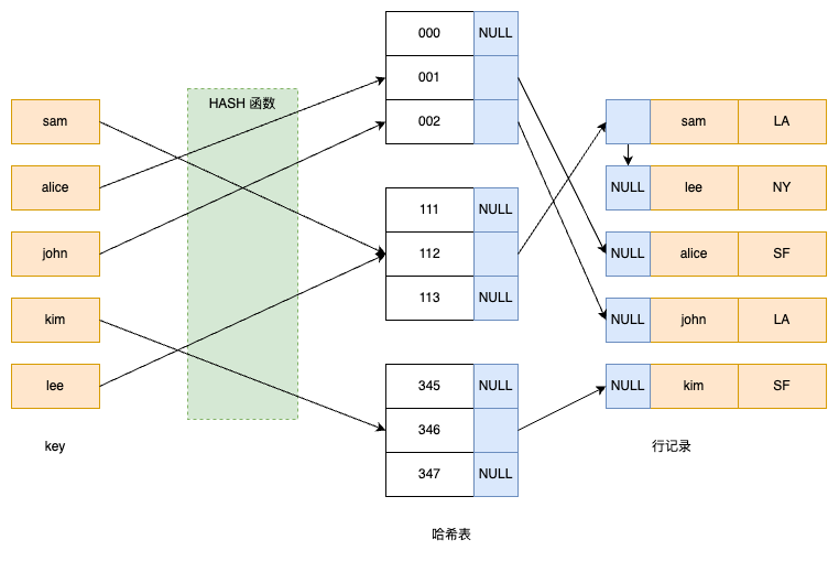
InnoDB 中的哈希算法

哈希表基本结构与冲突解决

• InnoDB 在缓冲池中维护一个哈希表，用于物理页号 → 缓冲池页地址的快速映射。
• 哈希冲突时采用链表方式：每个缓冲池页有一个指向同一哈希值下链上下一个页的指针，形成冲突链。

哈希函数：除法散列法（Division Method）

• InnoDB 选取的哈希函数为 除法散列，即：
  $hash_value  =  K   mod   m$ 其中，
  • K 是查询页标识的整数键；
  • m 是哈希表大小（槽位数）。
• 为了尽量均匀分布并减少冲突，InnoDB 通常将 m 选为略大于 缓冲池页总数 × 2 的质数。
  • 例如，若 innodb_buffer_pool_size = 10 MB，则缓冲池中总页数约为 $10MB÷16KB=640$ 页。
  • 按 2 倍页数原则，需要 $640×2=1280$ 个槽位，但 1280 不是质数，于是取下一个比 1280 稍大的质数 1399 作为哈希表槽数。

构造查询键 K

• InnoDB 中，每个页都有两个重要标识：
  1. space_id：表示该页所属的表空间（tablespace）编号；
  2. offset：表示该页在表空间内的偏移量（即第几个 16 KB 页）。
• InnoDB 将这两个值合并成一个整数键 K，其计算公式通常为：$K  =  (space_id  ≪  20)  +  offset$。
• 得到的 K 用于与哈希表槽数 m 做除法取余运算，确定该页在哈希表中对应的槽。

哈希索引

该索引采用哈希算法把键值换算成新的 hash 值，映射到对应的位置上，然后存储在 hash 表中。

• 特点
  • 只能用于对等比较（=，in），不支持范围查询（between，>，<，…）；
  • 无法利用索引完成排序操作；
  • 查询效率高，通常只需要一次索引就可以了，效率通常要高于 B+Tree 索引（不发生 hash 冲突的情况下）。
• 存储引擎支持
  • 支持 hash 索引的是 Memory 和 NDB 存储引擎，而 InnoDB 中具有自适应 hash 索引。

Hash 索引和 B+ 树索引的区别

1. B+ 树索引可以进行范围查询，Hash 索引不能。
2. B+ 树索引支持联合索引的最左侧原则，Hash 索引不支持。
3. B+ 树索引支持 order by 排序，Hash 索引不支持。
4. B+ 树使用 like 进行模糊查询的时候，LIKE ‘abc%’ 的话可以起到索引优化的作用，Hash 索引无法进行模糊查询。
5. Hash 索引在等值查询上比 B+ 树索引效率更高。

自适应哈希索引

自适应哈希索引（Adaptive Hash Index，AHI）是 InnoDB 存储引擎在运行时自动创建的一种轻量级哈希结构，用于加速对 B+ 树叶子页中热点记录的等值查找。InnoDB 会监测查询模式，一旦检测到某个叶子页或某条索引项的访问频率过高，便在 Buffer Pool 中为该叶子页构造哈希表节点，使后续对该页的等值查找可以通过哈希函数直接定位，而无需再遍历 B+ 树路径。

适用场景

• 等值查询：AHI 仅对形如 SELECT * FROM table WHERE indexed_col = constant 的等值匹配操作有效。如果是范围查询（BETWEEN、>, < 等）或排序（ORDER BY）、模糊匹配（LIKE ‘%…%’），则不能使用 AHI，只能回退到常规的 B+ 树扫描或其他索引操作。
• 热点数据页：在大表中，如果某个 B+ 树叶子页承载了大量相同或相近的等值访问（例如同一个二级索引项被频繁查询），AHI 能极大减少 B+ 树遍历的层级开销，将随机 I/O 降低为直接在内存哈希表查找。

全文检索

MySQL 的全文检索（Full-Text Search）功能主要基于倒排索引实现，在 MyISAM 和 InnoDB 存储引擎中均提供了不同的支持方式。其核心原理是在数据写入时将文本字段拆分成词汇单元，并建立一个词–文档或词–行号的映射表，从而使得在查询时能够快速检索包含指定关键词的记录。虽然 MySQL 的全文检索功能对于轻量级应用已经十分实用，但与专业搜索引擎（如 Lucene、Solr、Elasticsearch 等）相比，功能较为基础。

创建索引的注意点

• 使用合适的列作为索引
  • 经常作为查询条件（WHERE 子句）、排序条件（ORDER BY 子句）、分组条件（GROUP BY 子句）的列是建立索引的好候选。
  • 区分度低（唯一值比例低）的字段，例如性别，不要建索引。
  • 频繁更新的字段，不要作为主键或者索引。
  • 不建议用无序的值(例如身份证、UUID )作为索引，当主键具有不确定性，会造成叶子节点频繁分裂，出现磁盘存储的碎片化。
• 避免过多的索引
  • 每个索引都需要占用额外的磁盘空间。
  • 更新表（INSERT、UPDATE、DELETE 操作）时，所有的索引都需要被更新。
  • 维护索引文件需要成本；还会导致页分裂，IO 次数增多。
• 利用前缀索引和索引列的顺序
  • 对于字符串类型的列，可以考虑使用前缀索引来减少索引大小。
  • 在创建复合索引时，应该根据查询条件将最常用作过滤条件的列放在前面。

使用索引的注意点

• 最左前缀法则
  • 如果索引了多列（联合索引），要遵循最左前缀法则。最左前缀法则指的是查询从索引的最左列开始，并且不跳过索引中的列。如果跳过了某一列，索引将部分失效（后面的字段索引失效）。
• 范围查询
  • 联合索引中出现范围查询（>, <），范围查询右侧的列索引失效。因为范围查询会存在一次性获取大量符合条件的指针，这些指针指向 B+ 树中的子节点。这些子节点中都可能会包含右侧的列索引键，因此无法使用索引。规避方法：业务允许的情况下，使用 >=, <=。
• 索引列运算：在索引列上进行运算操作（各种函数），索引将失效。
• 字符串不加引号：使用字符串类型字段时，不加引号（会造成隐式类型转换），索引将失效。
• 模糊查询：如果仅仅是尾部模糊匹配，索引不会失效，如果是头部模糊匹配，索引失效。因为索引无法确定开头部分是什么内容。
• or 连接的条件：用 or 分割开的条件，如果 or 前面的条件中的列有索引，而后面的列中没有索引，那么涉及的索引都不会被用到。
• 数据分布的影响
  • 如果 MySQL 评估使用索引比全表更慢，则不使用索引。
  • 如果某个数据占比小，那么使用索引；否则，使用全表查询。

索引设计原则

1. 数据量较大（数据行超过 1M 条），查询操作频繁的表建立索引。
2. 经常作为查询条件（where），排序（order by），分组（group by）操作的字段建立索引。
3. 区分度高的列建立索引（区分度高，索引效率高）。
4. 长字符串、大文本字段建立前缀索引。
5. 尽量使用联合索引（覆盖索引），减少单列索引，避免回表。
6. 控制索引数量，维护大量索引代价高。
7. 如果索引列不能存储 NULL 值，请对其使用 NOT NULL 约束（方便优化器确定哪个索引更高效）。

索引失效的情况

• 在索引列上使用函数或表达式，索引可能无法使用，因为数据库无法预先计算出函数或表达式的结果。例如：SELECT * FROM table_name WHERE YEAR(date_column) = 2021。
• 使用不等于（<>）或者 NOT 操作通常会使索引失效，因为它们会扫描全表。
• 如果 LIKE 的模式串是以“%”或者“_”开头的，那么索引也无法使用。例如：SELECT * FROM table_name WHERE column LIKE '%abc'。
• 如果查询条件中使用了 OR，并且 OR 两边的条件分别涉及不同的索引，那么这些索引可能都无法使用。
• 如果 MySQL 估计使用全表扫描比使用索引更快时（通常是小表或者大部分行都满足 WHERE 子句），也不会使用索引。
• 联合索引不满足最左前缀原则时，索引会失效。

百万级别以上的数据如何删除？

先删除索引，然后删除其中的无用数据，删除完成后重新创建索引。

MySQL 数据库和 InnoDB 存储引擎表的各种类型文件如下：

参数文件：告诉 MySQL 实例启动时在哪里可以找到数据库文件，并且指定某些初始化参数，这些参数定义了某种内存结构的大小等设置，还会介绍各种参数的类型。

日志文件：用来记录 MySQL 实例对某种条件做出响应时写入的文件，如错误日志文件、二进制日志文件、慢查询日志文件、查询日志文件等。

socket 文件：当用 UNIX 域套接字方式进行连接时需要的文件。

pid 文件：MySQL 实例的进程 ID 文件。

MySQL 表结构文件：用来存放 MySQL 表结构定义文件。

存储引擎文件：由于 MySQL 表存储引擎的关系，每个存储引擎都会有自己的文件来保存各种数据。这些存储引擎真正存储了记录和索引等数据。本章主要介绍与 InnoDB 有关的存储引擎文件。

参数文件

当 MySQL 实例启动时，数据库会先去读一个配置参数文件，用来寻找数据库的各种文件所在位置以及指定某些初始化参数，这些参数通常定义了某种内存结构有多大等。在默认情况下，MySQL 实例会按照一定的顺序在指定的位置进行读取，用户只需通过命令 mysql –help | grep my.cnf 来寻找即可。

MySQL 实例可以不需要参数文件，这时所有的参数值取决于编译 MySQL 时指定的默认值和源代码中指定参数的默认值。但是，如果 MySQL 实例在默认的数据库库目录下找不到 mysql 系统数据库，则启动同样会失败。

参数类型

MySQL 数据库中的参数可以分为两类：

• 动态（dynamic）参数
• 静态（static）参数

动态参数意味着可以在 MySQL 实例运行中进行更改，静态参数说明在整个实例生命周期内都不得进行更改，就好像是只读（read only）的。可以通过 SET 命令对动态参数值进行修改，SET 的语法如下：

1
2
3

SET
[GLOBAL | SESSION] system_var_name = expr
| [@@GLOBAL. | @@SESSION.] system_var_name = expr;

这里可以看到 GLOBAL 和 SESSION 关键字，它们表明该参数的修改是基于当前会话还是整个实例的生命周期。有些动态参数只能在会话中进行修改，如 autocommit；而有些参数修改完后，在整个实例生命周期中都会生效，如 binlog_cache_size；而有些参数既可以在会话中又可以在整个实例的生命周期内生效，如 read_buffer_size。

对变量的全局值进行了修改，在这次的实例生命周期内都有有效，但 MySQL 实例本身并不会对参数文件中的该值进行修改。也就是说，在下次启动时 MySQL 实例还是会读取参数文件。若想在数据库实例下一次启动时该参数还是保留为当前修改的值，那么用户必须去修改参数文件。

日志文件

MySQL 中常见的日志文件有：

• 错误日志
• 二进制日志
• 慢查询日志
• 查询日志

错误日志

错误日志文件对 MySQL 的启动、运行、关闭过程进行了记录。用户在遇到问题时应该首先查看该文件以便定位问题。该文件不仅记录了所有的错误信息，也记录一些警告信息或正确的信息。用户可以通过命令 SHOW VARIABLES LIKE ‘log_error’ 来定位该文件。

1
2
3
4
5
6
7

[mysql]> show variables like 'log_error';

| Variable_name | Value              |
| ------------- | ------------------ |
| log_error     | ./Yihang.local.err |

1 row in set (0.07 sec)

慢查询日志

慢查询日志（slow log）可帮助用户定位可能存在问题的 SQL 语句，从而进行 SQL 语句层面的优化。例如，可以在 MySQL 启动时设一个阈值，将运行时间超过该值的所有 SQL 语句都记录到慢查询日志文件中。用户每天或每过一段时间对其进行检查，确认是否有 SQL 语句需要进行优化。该阈值可以通过参数 long_query_time 来设置，默认值为 10，代表 10 秒。

这里有两点需要注意。首先，设置 long_query_time 这个阈值后，MySQL 数据库会记录运行时间超过该值的所有 SQL 语句，但运行时间正好等于 long_query_time 的情况并不会被记录。也就是说，在源代码中判断的是大于 long_query_time，而非大于等于。

其次，从 MySQL 5.1 开始，long_query_time 开始以微秒记录 SQL 语句运行的时间，此前仅用秒为单位记录。而这样可以更精确地记录 SQL 的运行时间。对用户来说，一条 SQL 语句运行 0.5 秒和 0.05 秒是非常不同的，前者可能已经进行了表扫描，后者可能只是进行了索引查找。

另一个和慢查询日志有关的参数是 log_queries_not_using_indexes，如果运行的 SQL 语句没有使用索引，则 MySQL 同样会将这条 SQL 语句记录到慢查询日志文件。

MySQL 5.6.5 版本开始新增了一个参数 log_throttle_queries_not_using_indexes，用来表示每分钟允许记录到 slow log 的且未使用索引的 SQL 语句的最大次数。该参数默认值为 0，表示没有限制。在生产环境下，如果有大量未使用索引的查询，此类 SQL 会频繁地被记录到 slow log，从而导致日志文件持续膨胀。

用户可以通过慢查询日志找出有问题的 SQL 语句并进行优化。然而，随着 MySQL 服务器运行时间的增加，可能会有越来越多的查询被记录到慢查询日志，此时直接阅读日志文件就显得不够直观。MySQL 提供的 mysqldumpslow 工具可以很好地帮助 DBA 对慢查询日志进行汇总和分析。

MySQL 5.1 开始可以将慢查询的日志记录放入一张表中，这使得用户的查询更加方便和直观。

InnoSQL 版本加强了对于 SQL 语句的捕获方式。在原版 MySQL 的基础上在 slow log 中增加了对逻辑读取（logical reads）和物理读取（physical reads）的统计。这里的物理读取是指从磁盘进行 IO 读取的次数，逻辑读取包含所有的读取，不管是磁盘还是缓冲池。

用户可以通过额外的参数 long_query_io 将超过指定逻辑 IO 次数的 SQL 语句记录到 slow log 中。该值默认为 100，即表示对于逻辑读取次数大于 100 的 SQL 语句，记录到 slow log 中。

查询日志

查询日志记录了所有对 MySQL 数据库请求的信息，无论这些请求是否得到了正确的执行。默认文件名为：<主机名>.log。

二进制日志

二进制日志（binary log）记录了对 MySQL 数据库执行更改的所有操作，但是不包括 SELECT 和 SHOW 这类操作，因为这类操作对数据本身并没有修改。然而，若操作本身并没有导致数据库发生变化，那么该操作可能也会写入二进制日志，但是这种情况只会发生在 binlog_format 参数的值为 ROW 的情况下。

Statement-Based Logging (SBL) 下，所有 DML/DDL 语句均写入二进制日志，无论它们是否实际修改了任何行。

Row-Based Logging (RBL) 下，只有真正产生行变更的事件才写入二进制日志；如果一条语句对零行生效，就不会产生相应的行事件。

如果用户想记录 SELECT 和 SHOW 操作，那只能使用查询日志，而不是二进制日志。此外，二进制日志还包括了执行数据库更改操作的时间等其他额外信息。总的来说，二进制日志主要有以下几种作用：

• 恢复（recovery）：某些数据的恢复需要二进制日志，例如，在一个数据库全备文件恢复后，用户可以通过二进制日志进行 point-in-time 的恢复。
• 复制（replication）：其原理与恢复类似，通过复制和执行二进制日志使一台远程的 MySQL 数据库（一般称为 slave 或 standby）与一台 MySQL 数据库（一般称为 master 或 primary）进行实时同步。
• 审计（audit）：用户可以通过二进制日志中的信息进行审计，判断是否有对数据库进行注入的攻击。

以下配置文件的参数影响着二进制日志记录的信息和行为：

• max_binlog_size
• binlog_cache_size
• sync_binlog
• binlog-do-db
• binlog-ignore-db
• log-slave-update
• binlog_format

参数 max_binlog_size 指定了单个二进制日志文件的最大值，如果超过该值，则产生新的二进制日志文件，后缀名加 1，并记录到 .index 文件。从 MySQL 5.0 开始的默认值为 1073741824，代表 1 G（在之前版本中 max_binlog_size 默认大小为 1.1 G）。

当使用事务的存储引擎（如 InnoDB 存储引擎）时，所有未提交（uncommitted）的二进制日志会被记录到一个缓冲中去，等该事务提交（committed）时再将缓冲中的二进制日志写入二进制日志文件，而该缓冲的大小由 binlog_cache_size 决定，默认大小为 32K。此外，binlog_cache_size 是基于会话（session）的，也就是说，当一个线程开始一个事务时，MySQL 会自动分配一个大小为 binlog_cache_size 的缓冲，因此该值的设置需要相当小心，不能设置过大。当一个事务的记录大于设置的 binlog_cache_size 时，MySQL 会把缓冲中的日志写入一个临时文件中，因此该值又不能设置得过小。

在默认情况下，二进制日志并不是在每次写的时候同步到磁盘（用户可以理解为缓冲写）。因此，当数据库所在操作系统发生宕机时，可能会有最后一部分数据没有写入二进制日志文件中，这会给恢复和复制带来问题。参数 sync_binlog=[N] 表示每写缓冲多少次就同步到磁盘。如果将 N 设为 1，即 sync_binlog=1 表示采用同步写磁盘的方式来写二进制日志，这时写操作不再使用操作系统的缓冲来写二进制日志。sync_binlog 的默认值为 0，如果使用 InnoDB 存储引擎进行复制，并且想得到最大的高可用性，建议将该值设为 1。不过该值为 0 时，的确会对数据库的 I/O 系统带来一定的影响。

但是，即使将 sync_binlog 设为 1，还是会有一种情况导致问题的发生。当使用 InnoDB 存储引擎时，在一个事务发出 COMMIT 动作之前，由于 sync_binlog=1，因此会将二进制日志立即写入磁盘。如果这时已经写入了二进制日志，但是提交还没有发生，并且此时发生了宕机，那么在 MySQL 数据库下次启动时，由于 COMMIT 操作并没有发生，这个事务会被回滚。但是二进制日志已经记录了该事务信息，不能被回滚。这个问题可以通过将参数 innodb_support_xa 设为 1 来解决，虽然 innodb_support_xa 与 XA 事务有关，但它同时也确保了二进制日志和 InnoDB 存储引擎数据文件的同步。

参数 binlog-do-db 和 binlog-ignore-db 表示需要写入或忽略写入哪些库的日志。默认为空，表示需要同步所有库的日志到二进制日志。

如果当前数据库是复制中的 slave 角色，则它不会将从 master 取得并执行的二进制日志写入自己的二进制日志文件中去。如果需要写入，要设置 log-slave-update。如果需要搭建 master⇒slave⇒slave 架构的复制，则必须设置该参数。

binlog_format 参数十分重要，它影响了记录二进制日志的格式。在 MySQL 5.1 版本之前，没有这个参数，因此所有二进制日志文件的格式都是基于 SQL 语句（statement）级别的。同时，对于复制也有一定要求。例如在主服务器上运行 rand、uuid 等函数，或者使用触发器等操作，这些都可能会导致主从服务器上表中数据的不一致（not sync）。另一个影响是，你会发现 InnoDB 存储引擎的默认事务隔离级别是 REPEATABLE READ。这其实也是因为二进制日志文件格式的关系：如果使用 READ COMMITTED 的事务隔离级别，会出现类似“丢失更新”的现象，从而导致主从数据库上的数据不一致。具体细节如下：

存在表 t1，定义如下：

1
2
3
4
5
6

CREATE TABLE t1 (
   a int(11) DEFAULT NULL, 
   b int(11) DEFAULT NULL, 
   KEY a (a) 
  ) ENGINE=InnoDB DEFAULT CHARSET=latin1; 
insert into t1 values(10,2),(20,1);

接着开始执行两个事务的写操作：

以上两个事务执行之后，数据库里面的记录会变成（11，2）和（20，2）。

因为事务的隔离级别是 read committed，所以，事务 1 在更新时，只会对 b = 2 这行加上行级锁，不会影响到事务 2 对 b = 1 这行的写操作。

以上两个事务执行完成之后，会在 binlog 中记录两条记录，因为事务 2 先提交，所以 UPDATE t1 SET b=2 where b=1; 会被优先记录，然后再记录 UPDATE t1 SET a=11 where b=2;。

binlog 同步到备从库之后，SQL语句回放时，会先执行 UPDATE t1 SET b=2 where b=1;，再执行 UPDATE t1 SET a=11 where b=2;。

这时候，数据库中的数据就会变成（11，2）和（11，2）。这就导致主库和备库的数据不一致了！！！

为了避免这种问题的发生，MySQL 就把数据库的默认隔离级别设置成了 Repeatable Read。

因为 Repetable Read 下，MySQL 在更新数据的时候不仅对更新的行加行级锁，还会增加 gap lock。同样是上面的例子，在事务 2 执行的时候，因为事务 1 增加了 gap lock，就会导致事务执行被卡住，需要等事务 1 提交或者回滚后才能继续执行。

除了设置默认的隔离级别外，MySQL 还在当使用 STATEMENT 格式的 binlog 的情况下，禁止设置 READ COMMITTED 作为事务隔离级别。

MySQL 5.1 开始引入了 binlog_format 参数，该参数可设的值有：STATEMENT、ROW 和 MIXED。

(1) STATEMENT 格式：二进制日志文件记录的是日志的逻辑 SQL 语句。

(2) ROW 格式下，二进制日志记录的不再是简单的 SQL 语句了，而是记录表的行更改情况。同时，对上述提及的 STATEMENT 格式下复制的问题予以解决。从 MySQL 5.1 版本开始，如果设置了 binlog_format 为 ROW，可以将 InnoDB 的事务隔离级别设为 READ COMMITTED，以获得更好的并发性。

(3) MIXED 格式下，MySQL 默认采用 STATEMENT 格式进行二进制日志文件的记录，但是在一些情况下会使用 ROW 格式，可能的情况有：

• 使用了 UUID()、USER()、CURRENT_USER()、FOUND_ROWS()、ROW_COUNT() 等不确定函数。
• 使用了 INSERT DELAY 语句。
• 使用了用户定义函数（UDF）。
• 使用了临时表（temporary table）。

binlog_format 是动态参数，因此可以在数据库运行环境下进行更改。当然，也可以将全局的 binlog_format 设置为想要的格式，不过通常这个操作会带来问题，运行时要确保更改后不会对复制带来影响。在通常情况下，我们将参数 binlog_format 设置为 ROW，这可以为数据库的恢复和复制带来更好的可靠性。但是不能忽略的一点是，这会带来二进制文件大小的增加，有些语句下的 ROW 格式可能需要更大的容量。也就是说将参数 binlog_format 设置为 ROW，会对磁盘空间要求有一定的增加。而由于复制是采用传输二进制日志方式实现的，因此复制的网络开销也有所增加。

二进制日志文件的文件格式为二进制（好像有点废话），不能像错误日志文件、慢查询日志文件那样用 cat、head、tail 等命令来看查看。要查看二进制日志文件的内容，必须通过 MySQL 提供的工具 mysqlbinlog。

示例：

执行的 SQL 为：UPDATE users SET age = age + 1 WHERE id = 100;

binlog_format=STATEMENT 时的 binlog 输出（可读）：

1
2
3
4

# at 234
#240523 15:00:01 server id 1 end_log_pos 345 Query  thread_id=7 exec_time=0 error_code=0
SET TIMESTAMP=1716495601/*!*/;
UPDATE users SET age = age + 1 WHERE id = 100/*!*/;

binlog_format=ROW 时的 binlog 输出（不可读）：

1
2
3
4
5
6
7
8
9
10
11

# at 456
#240523 15:00:02 server id 1 end_log_pos 567 Table_map: `test`.`users` mapped to number 108
# at 567
#240523 15:00:02 server id 1 end_log_pos 678 Update_rows: table id 108 flags: STMT_END_F
### UPDATE `test`.`users`
### WHERE
###  @1=100 /* id */
###  @2=20 /* age (原值) */
### SET
###  @1=100
###  @2=21 /* age (新值) */

因此，在 ROW 格式下，binlog 中对于一个简单的更新操作记录了整个行额所有字段的更改信息。这也解释了为什么 ROW 格式下的 binlog 对磁盘空间要求有一定的增加。

套接字文件

在 UNIX 系统下本地连接 MySQL 可以采用 UNIX 域套接字方式，这种方式需要一个套接字（socket）文件。套接字文件可由参数 socket 控制。一般在 /tmp 目录下，名为 mysql.sock。

pid 文件

当 MySQL 实例启动时，会将自己的进程 ID 写入一个文件中——该文件即为 pid 文件并且可由参数 pid_file 控制，默认位于数据库目录下，文件名为主机名 .pid。

表结构定义文件

因为 MySQL 插件式存储引擎的体系结构的关系，MySQL 数据的存储是根据表进行的，每个表都会有与之对应的文件。但不论表采用何种存储引擎，MySQL 都有一个以 .frm 为后缀名的文件，这个文件记录了该表的表结构定义。

.frm 还用来存放视图的定义，如用户创建了一个 v_a 视图，那么对应地会产生一个 v_a.frm 文件，用来记录视图的定义。该文件是文本文件，可以直接使用 cat 命令进行查看。

InnoDB 存储引擎文件

之前介绍的文件都是 MySQL 数据库本身的文件，和存储引擎无关。除了这些文件外，每个表存储引擎还有其自己独有的文件，包括重做日志文件、表空间文件。

表空间文件

InnoDB 采用将存储的数据按表空间（tablespace）进行存放的设计。在默认配置下会有一个初始大小为 10MB，名为 ibdata1 的文件。该文件就是默认的表空间文件（tablespace file），用户可以通过参数 innodb_data_file_path 对其进行设置，格式如下：

1

innodb_data_file_path=datafile_spec1[;datafile_spec2]...

用户可以通过多个文件组成一个表空间，同时制定文件的属性，如：

1

innodb_data_file_path = /db/ibdata1:2000M;/dr2/db/ibdata2:2000M:autoextend

这里将 /db/ibdata1 和 /dr2/db/ibdata2 两个文件用于组成表空间。若这两个文件位于不同的磁盘上，磁盘的负载可能被平均，因此可以提高数据库的整体性能。同时，两个文件的文件名后都跟了属性，表示文件 ibdata1 的大小为 2000MB，文件 ibdata2 的大小为 2000MB，如果用完了这 2000MB，该文件可以自动增长（autoextend）。

设置 innodb_data_file_path 参数后，所有基于 InnoDB 存储引擎的表的数据都会记录到该共享表空间中。若设置了参数 innodb_file_per_table，则用户可以将每个基于 InnoDB 存储引擎的表生成一个独立表空间。独立表空间的命名规则为：表名 .ibd。需要注意的是，这些单独的表空间文件仅存储该表的数据、索引和插入缓冲 BITMAP 等信息，其余信息还是存放在默认的表空间中。

下图展示了 InnoDB 对于文件的存储方式：

Redo 日志文件

在默认情况下，在 InnoDB 存储引擎的数据目录下会有两个名为 ib_logfile0 和 ib_logfile1 的文件。

当实例或介质失败时，重做日志文件就能派上用场。例如，数据库由于所在主机掉电导致实例失败，InnoDB 存储引擎会使用 Redo 日志恢复到掉电前的时刻，以此来保证数据的完整性。

每个 InnoDB 存储引擎至少有 1 个 Redo 日志文件组，每个文件组下至少有 2 个 Redo 日志文件，如默认的 ib_logfile0 和 ib_logfile1。为了得到更高的可靠性，用户可以设置多个镜像日志组，将不同的文件组放在不同的磁盘上，以此提高 Redo 日志的高可用性。在日志组中每个 Redo 日志文件的大小一致，并以循环写入的方式运行。InnoDB 存储引擎先写 Redo 日志文件 1，当达到文件的最后时，会切换至 Redo 日志文件 2，再当重做日志文件 2 也被写满时，会再切换到 Redo 日志文件 1 中。

下列参数影响着 Redo 日志文件的属性：

• innodb_log_file_size
• innodb_log_files_in_group
• innodb_mirrored_log_groups
• innodb_log_group_home_dir

参数 innodb_log_file_size 指定每个 Redo 日志文件的大小。在 InnoDB 1.2.x 版本之前，Redo 日志文件总的大小不得大于等于 4GB，而 1.2.x 版本将该限制扩大为了 512GB。

参数 innodb_log_files_in_group 指定了日志文件组中 Redo 日志文件的数量，默认为 2。

参数 innodb_mirrored_log_groups 指定了日志镜像文件组的数量，默认为 1，表示只有一个日志文件组，没有镜像。若磁盘本身已经做了高可用的方案，如磁盘阵列，那么可以不开启 Redo 日志镜像的功能。

最后，参数 innodb_log_group_home_dir 指定了日志文件组所在路径，默认为 ./，表示在 MySQL 数据库的数据目录下。

Redo 日志文件的大小设置对于 InnoDB 存储引擎的性能有着非常大的影响。一方面 Redo 日志文件不能设置得太大，如果设置得很大，在恢复时可能需要很长的时间；另一方面又不能设置得太小了，否则可能导致一个事务的日志需要多次切换 Redo 日志文件。此外，Redo 日志文件太小会导致频繁地发生 async checkpoint，导致性能的抖动。因为，如果 Redo 日志文件大小超过最大容量则必须将缓冲池中脏页列表（flush list）中的部分脏数据写回磁盘，这时会导致用户线程的阻塞。

Redo 日志和二进制日志有什么区别？

首先，二进制日志会记录所有与 MySQL 数据库有关的日志记录，包括 InnoDB、MyISAM、Heap 等其他存储引擎的日志。而 InnoDB 存储引擎的 Redo 日志只记录有关该存储引擎本身的事务日志。

其次，记录的内容不同。无论用户将二进制日志文件记录的格式设为 STATEMENT 还是 ROW，又或者是 MIXED，其记录的都是关于一个事务的具体操作内容，即该日志是逻辑日志。而 InnoDB 存储引擎的 Redo 日志文件记录的是关于每个页（Page）的更改的物理情况。

此外，写入的时间也不同，二进制日志文件仅在事务提交前进行提交，即只写磁盘一次，不论这时该事务多大。而在事务进行的过程中，却不断有 Redo 日志条目（redo entry）被写入到 Redo 日志文件中。

Redo 日志条目的结构如下：

上图中 Redo 日志条目是由 4 个部分组成：

• redo_log_type 占用 1 字节，表示重做日志的类型。
• space 表示表空间的 ID，但采用压缩的方式，因此占用的空间可能小于 4 字节。
• page_no 表示页的偏移量，同样采用压缩的方式。
• redo_log_body 表示每个重做日志的数据部分，恢复时需要调用相应的函数进行解析。

写入重做日志文件的操作不是直接写，而是先写入一个重做日志缓冲中，然后按照一定的条件顺序地写入日志文件。下图是 Redo 日志的写入过程：

从重做日志缓冲往磁盘写入时是按 512 字节，也就是一个扇区的大小进行写入。因为在传统的磁盘存储设备中，扇区是最小的物理写入单位。当操作系统或数据库系统请求写入数据时，磁盘控制器会确保整个扇区的数据要么被完整地写入，要么在发生故障（如断电）时不进行任何写入。这种机制确保了写入操作的原子性，即不会出现撕裂写（torn write）的情况，因此在重做日志的写入过程中不需要有 doublewrite。

前面提到了从日志缓冲写入磁盘上的重做日志文件是按一定条件进行的，那这些条件有哪些呢？我们知道在主线程中每秒会将重做日志缓冲写入磁盘的重做日志文件中，不论事务是否已经提交。另一个触发写磁盘的过程是由参数 innodb_flush_log_at_trx_commit 控制，表示在提交操作时，处理重做日志的方式。

参数 innodb_flush_log_at_trx_commit 的有效值有 0、1、2。

0 代表当提交事务时，并不将事务的重做日志写入磁盘上的日志文件，而是等待主线程每秒的刷新。1 和 2 不同的地方在于：

• 1 表示在执行 commit 时将重做日志缓冲同步写到磁盘，即伴有 fsync 的调用。
• 2 表示将重做日志异步写到磁盘，即写到文件系统的缓存中。因此不能完全保证在执行 commit 时肯定会写入重做日志文件，只是有这个动作发生。

因此为了保证事务的 ACID 中的持久性，必须将 innodb_flush_log_at_trx_commit 设置为 1，也就是每当有事务提交，就必须确保事务已经写入重做日志文件。那当数据库因为意外发生宕机时，可以通过重做日志文件恢复，并保证可以恢复已经提交的事务。

而将重做日志文件设置为 0 或 2，都有可能发生恢复时部分事务的丢失。不同之处在于，设置为 2 时，当 MySQL 数据库发生宕机而操作系统及服务器并没有发生宕机时，由于此时未写入磁盘的事务日志保存在文件系统缓存中，当恢复时同样能保证数据不丢失。

/usr/local/mysql/bin 目录下提供了多个客户端工具，具体如下：

MySQL 在每个实例中都预装了四个系统数据库，用于存储元数据、权限及运行时性能统计等信息。information_schema 以视图形式提供数据字典和权限信息的只读访问；mysql 模式包含用户账户、时区、复制配置等必要的系统表；performance_schema 聚焦于运行时性能监控，采用专用存储引擎记录服务器内部执行情况；而 sys 模式则封装了一系列基于 performance_schema 的视图和存储过程，帮助 DBA 和开发人员快速诊断与调优。

与系统数据库配套，MySQL Server 安装包中还包括多种命令行工具：

• mysql：交互式 SQL Shell，支持命令行编辑及脚本化操作，用于执行任意 SQL 语句，并以可读的格式显示结果。
• mysqladmin：管理型客户端，可检查服务器状态、创建/删除数据库、执行刷新及关闭操作等。
• mysqlbinlog：二进制日志处理工具，可查看或导出 binlog、relay log，常用于增量备份与故障恢复。
• mysqlshow：快速展示已有数据库、表及字段信息，相当于对 SHOW 系列语句的轻量封装。
• mysqldump：生成逻辑备份的主力工具，将库表结构和数据导出为 SQL 脚本或其他格式，用于迁移和恢复 。
• mysqlimport：将文本文件批量导入到表中，通常与 mysqldump -T 导出的数据配合使用。
• mysqlcheck：表维护工具，可检查、修复、优化和分析表，用于日常健康检查与性能优化。
• source（MySQL 客户端内置命令）：在 mysql> 提示符下执行指定的 .sql 文件，常用于批量恢复脚本。

Data Model and Performance Metrics

1. ER Diagram and Database Design

• ER Diagram (Figure 1.a):Represents entities and relationships in the BG system.
  • Member Entity:
    • Represents users with a registered profile, including a unique ID and a set of adjustable-length string attributes to create records of varying sizes.
    • Each user can have up to two images:
      • Thumbnail Image: Small (in KBs), used for displaying in friend lists.
      • High-Resolution Image: Larger (hundreds of KBs or MBs), displayed when visiting a user profile.
      • Using thumbnails significantly reduces system load compared to larger images.
  • Friend Relationship:
    • Captures relationships or friend requests between users. An attribute differentiates between invitations and confirmed friendships.
  • Resource Entity:
    • Represents user-owned items like images, questions, or documents. Resources must belong to a user and can be posted on their profile or another user’s profile.
  • Manipulation Relationship:
    • Manages comments and restrictions (e.g., only friends can comment on a resource).

2. BG Workload and SLA (Service-Level Agreement)

• Workload: BG supports defining workloads at the granularity of:

  • Actions: Single operations like “view profile” or “list friends.”
  • Sessions: A sequence of related actions (e.g., browsing a profile, sending a friend request).
  • Mixed Workloads: A combination of actions and sessions.

• Service-Level Agreement (SLA):

  • Goal: Ensures the system provides reliable performance under specified conditions.
  • Example SLA Requirements: SLA, e.g., 95% of requests to observe a response time equal to or faster than 100 msec with at most 0.1% of requests observing unpredictable data for 10 minutes.

• Metrics:

  • SoAR (Social Action Rating): Measures the highest number of actions per second that meet the SLA.
  • Socialites: Measures the maximum number of concurrent threads that meet the SLA, reflecting the system’s multithreading capabilities.

3. Performance Evaluation Example

• SQL-X System Performance:SQL-X is a relational database with strict ACID compliance.
  • Initially, throughput increases with more threads.
  • Beyond a certain threshold (e.g., 4 threads), request queuing causes response times to increase, reducing SLA compliance.
  • With 32 threads, 99.94% of requests exceed the 100-millisecond SLA limit, indicating significant performance degradation.

4. Concurrency and Optimization in BG

• Concurrency Management:

  • BG prevents two threads from emulating the same user simultaneously to realistically simulate user behavior.

• Unpredictable Data Handling:

  • Definition: Data that is stale, inconsistent, or invalid due to system limitations or race conditions.
  • Validation:
    • BG uses offline validation to analyze read and write logs.
    • It determines acceptable value ranges for data and flags any reads that fall outside these ranges as unpredictable.

If SoAR is zero, the data store fails to meet SLA requirements, even with a single-threaded BGClient issuing requests.

Actions

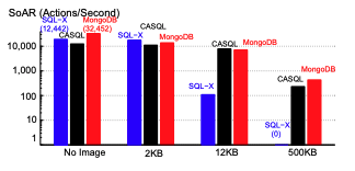
Performance Analysis of View Profile

Performance of VP is influenced by whether profile images are included and their sizes.

Experiment Setup:

• Profile data tested with:
• • No images.
  • 2 KB thumbnails combined with profile images of 2 KB, 12 KB, and 500 KB sizes.
• Metrics: SoAR (Social Action Rating) measures the number of VP actions per second that meet the SLA (response time ≤ 100 ms).

Results:

1. No Images:

   • MongoDB performed the best, outperforming SQL-X and CASQL by almost 2x.

2. 12 KB Images:

   • SQL-X’s SoAR dropped significantly, from thousands of actions per second to only hundreds.

3. 500 KB Images:

   • SQL-X failed to meet the SLA (SoAR = 0) because transmitting large images caused significant delays.

   • MongoDB and CASQL also experienced a decrease in SoAR but performed better than SQL-X.

Role of CASQL:

• CASQL outperformed SQL-X due to its caching layer (memcached):

  • During a warm-up phase, 500,000 requests populate the cache with key-value pairs for member profiles.

  • Most requests are serviced by memcached instead of SQL-X, significantly improving performance with larger images (12 KB and 500 KB).

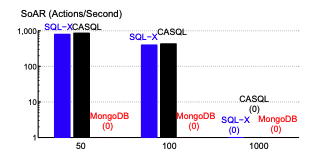
Performance Analysis of List Friends

1. SQL-X

• Process:
  • Joins the Friends table with the Members table to fetch the friend list.
  • Friendship between two members is represented as a single record in the Friends table.
• Performance:
  • When ϕ (number of friends) is 1000, SQL-X struggles due to the overhead of joining large tables and fails to meet SLA requirements.

2. CASQL

• Process:
  • Uses a memcached caching layer to store and retrieve results of the LF action.
  • Results are cached as key-value pairs.
• Performance:
  • Outperforms SQL-X when ϕ is 50 or 100 by a small margin (<10% improvement).
  • At ϕ=1000, memcached’s key-value size limit (1 MB) causes failures, as the data exceeds this limit.
  • Adjusting memcached to support larger key-value pairs (e.g., 2 MB for 1000 friends with 2 KB thumbnails) could improve performance.

3. MongoDB

• Process:
  • Retrieves the confirmedFriends array from the referenced member’s document.
  • Can fetch friends’ profile documents one by one or as a batch.
• Performance:
  • Performs no joins, but its SLA compliance is poor for larger friend counts.
  • SoAR is zero for ϕ=50,100,1000, as it fails to meet the 100 ms response time requirement.
  • For smaller friend lists (ϕ=10), MongoDB achieves a SoAR of 6 actions per second.

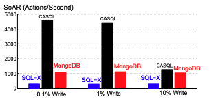
Mix of Read and Write Actions

• Purpose: Evaluates the performance of data stores under different ratios of read and write operations.
• Categories:
  • Read actions: Include operations like View Profile (VP), List Friends (LF), and View Friend Requests (VFR).
  • Write actions: Modify friendship relationships and invalidate cached key-value pairs (e.g., Invite Friend, Accept Friend Request).
• Mix Variations:
  • Very low writes (0.1%): Dominantly read-heavy workloads.
  • Low writes (1%): Slightly higher frequency of write actions.
  • High writes (10%): Write-intensive workloads.

Performance Analysis (Mix of Read and Write Actions)

• SoAR Comparison:
  • CASQL consistently achieves the highest SoAR for all write mixes due to its caching mechanism.
  • MongoDB outperforms SQL-X by a factor of 3 across all workloads.

Observations by Write Percentage:

1. 0.1% Writes (Read-Dominant):

   • CASQL significantly outperforms MongoDB due to efficient use of cached key-value pairs.

   • SQL-X lags due to the overhead of processing read actions directly from the RDBMS.

2. 1% Writes:

   • CASQL remains the best performer but shows sensitivity to increasing writes as it invalidates cached data, redirecting more queries to the RDBMS.

   • MongoDB maintains a consistent performance advantage over SQL-X.

3. 10% Writes (Write-Heavy):

   • CASQL slightly outperforms MongoDB, but the gap narrows due to the higher frequency of cache invalidations.

   • SQL-X continues to struggle with write-heavy workloads due to its lack of caching.

Session

Definition: A session is a sequence of actions performed by a socialite (user) in the social network.

Key Concepts:

1. Think Time: Delay between consecutive actions within a session.
2. Inter-Arrival Time: Delay between sessions initiated by different socialites.

Key Considerations

1. Dependencies:

   • Some sessions rely on specific database states (e.g., friends or pending requests).

   • For example, if m_i has no friends or pending requests, certain sessions terminate early.

2. Concurrency Handling:

   • BG uses in-memory data structures to simulate database states and prevent conflicts (e.g., multiple threads deleting the same comment).

   • Ensures integrity by managing semaphores and detecting unpredictable data.

3. Extensibility:

   • BG allows developers to define new sessions by combining different mixes of actions.

Parallelism

BG’s Scalable Benchmarking Framework

To address these limitations, BG employs a shared-nothing architecture with the following components:

1. BGCoord (Coordinator)

• Role: Oversees and coordinates the benchmarking process.
• Responsibilities:
  • Computes SoAR and Socialites ratings.
  • Assigns workloads to BGClients and monitors their progress.
  • Aggregates results (e.g., response times, throughput) for visualization.
• Process:
  • Splits the workload among N BGClients.
  • Ensures each BGClient works independently to prevent resource contention.

2. BGClient

• Role: Executes tasks assigned by BGCoord.
• Responsibilities:
  • Creates a database based on BG specifications.
  • Simulates workload actions and computes metrics like unpredictable data volume.
  • Periodically reports metrics to BGCoord for aggregation.

3. Visualization Deck

• Role: Provides a user interface for monitoring and controlling the benchmarking process.
• Features:
  • Allows users to configure parameters (e.g., SLA, workloads).
  • Visualizes the ratings (SoAR, Socialites) and progress of the benchmarking.

Scaling with BGClients

• Fragmentation:
  • The database is split into N logical fragments, each assigned to a BGClient.
  • Each fragment includes unique members, friendships, and resources, ensuring no overlap between BGClients.
• Decentralized D-Zipfian Distribution:
  • Used to balance workloads across nodes with different processing speeds.
  • Faster nodes handle larger fragments, ensuring equal workload completion times.

Unpredictable Data

Definition: Data that is stale, inconsistent, or invalid, produced due to race conditions, dirty reads, or eventual consistency.

BG’s Validation Process

Validation Implementation

1. Log Generation:
   • BG generates read log records (observed values) and write log records (new or delta values).
2. Offline Validation:
   • For each read log entry:
     • BG computes a range of valid values using overlapping write logs.
     • If the observed value is outside this range, it is flagged as unpredictable.

Impact of Time-to-Live (TTL) on Unpredictable Data

Results:

1. Higher TTL Increases Stale Data:

   • A higher TTL (e.g., 120 seconds) results in more stale key-value pairs, increasing the percentage of unpredictable data.

   • For T=100T = 100T=100, unpredictable data is:

     • ~79.8% with TTL = 30 seconds.
     • ~98.15% with TTL = 120 seconds.

2. Performance Trade-off:

   • A higher TTL improves performance (fewer cache invalidations) but increases stale data.

   • Lower TTL reduces stale data but impacts cache performance.

Heuristic Search for Rating

Why Use Heuristic Search?

• Exhaustive search starting from T=1 to the maximum T is time-consuming.
• MongoDB with T=1000 and Δ=10 minutes would take 7 days for exhaustive testing.

Steps in Heuristic Search:

1. Doubling Strategy:

   • Start with T=1, double T after each successful experiment.

   • Stop when SLA fails, narrowing down T to an interval.

2. Binary Search:

   • Identify the T corresponding to max throughput within the interval.

   • Used for both SoAR (peak throughput) and Socialites (maximum concurrent threads).

Questions

What system metrics does BG quantify?

SoAR (Social Action Rating):

• The highest throughput (actions per second) that satisfies a given SLA, ensuring at least α% of requests meet the response time β, with at most τ% of requests observing unpredictable data.

Socialites Rating:

• The maximum number of simultaneous threads (or users) that a data store can support while still meeting the SLA requirements.

Throughput:

• Total number of completed actions per unit of time.

Response Time:

• Average or percentile-based latency for each action.

Unpredictable Data:

• The percentage of actions that observe stale, inconsistent, or invalid data during execution.

How does BG scale to generate a large number of requests?

BG employs a shared-nothing architecture with the following mechanisms to scale effectively:

1. Partitioning Members and Resources:

   • BGCoord partitions the database into logical fragments, each containing a unique subset of members, their resources, and relationships.

   • These fragments are assigned to individual BGClients.

2. Multiple BGClients:

   • Each BGClient operates independently, generating workloads for its assigned logical fragment.

   • By running multiple BGClients in parallel across different nodes, BG can scale horizontally to handle millions of requests.

3. D-Zipfian Distribution:

   • To ensure realistic and scalable workloads, BG uses a decentralized Zipfian distribution (D-Zipfian) that dynamically assigns requests to BGClients based on node performance.

   • Faster nodes receive a larger share of the logical fragments, ensuring even workload distribution.

4. Concurrency Control:

   • BG prevents simultaneous threads from issuing actions for the same user, maintaining the integrity of modeled user interactions and avoiding resource contention.

If two modeled users, A and B, are already friends, does BG generate a friend request from A to B?

No, BG does not generate a friend request from A to B if they are already friends.

Before generating a friend request, BG validates whether the relationship between A and B is pending or already confirmed. For example, in the InviteFrdSession, BG only selects users who have no existing “friend” or “pending” relationship with the requester to receive a new friend request.

Reference: https://www.cidrdb.org/cidr2013/Papers/CIDR13_Paper93.pdf